Nonparametric versus parametric expected shortfall

R. Douglas Martin and Shengyu Zhang

Abstract

We use influence functions as a basic tool to study unconditional nonparametric and parametric expected shortfall (ES) estimators with regard to returns data influence, standard errors and coherence. Nonparametric ES estimators have a monotonically decreasing influence function of returns. ES maximum likelihood estimator (MLE) influence functions are nonmonotonic and approximately symmetric, resulting in large positive returns contributing to risk. However, ES MLEs have the lowest possible asymptotic variance among consistent ES estimators. Influence functions are used to derive large sample standard error formulas for both types of ES estimator for normal and t -distributions as well as to evaluate nonparametric ES estimator inefficiency. Monte Carlo results determine finite sample sizes for which the standard errors of both types of ES estimators are sufficiently accurate to be used in practice. The nonmonotonicity of ES MLEs leads us to study a modification of normal distribution MLEs in which standard deviation is replaced by semi-standard deviation (SSD). Influence function theory is used to establish a condition under which an SSD-based ES risk estimator has monotonic influence functions and the underlying risk measures are coherent. It is also shown that the SSD-based estimator’s asymptotic standard error is only slightly larger than that of the standard deviation-based estimator.

Download PDF Appendix 1

Introduction

1 Introduction

In recent years, expected shortfall (ES), which appeared in the risk literature as conditional value-at-risk (VaR) well over a decade ago, has been receiving increased attention. This is not surprising in view of ES’s intuitive appeal (it averages all the returns below VaR) and theoretical appeal (it is a coherent risk measure). A result of this increasing attention is that in 2013–14 the Basel Committee on Banking Supervision (BCBS) at the Bank for International Settlements (BIS) proposed to replace VaR by ES for Basel III (see Basel Committee on Banking Supervision 2013). More details may be found in Basel Committee on Banking Supervision (2014a,b). In view of those BIS recommendations, we can expect to see more extensive use of ES for risk management purposes with regard to capital adequacy as well as for portfolio construction.

With the above in mind, the purpose of this paper is to deepen our understanding of the statistical properties of unconditional ES estimators, henceforth referred to simply as ES estimators, in contrast to conditional ES estimators. An extensive literature exists on conditional ES (and conditional VaR), including early articles by McNeil and Frey (2000), Martins-Filho and Yao (2006) and Cai and Wang (2008) as well as a recent article by Martins-Filho et al (2018). Conditional ES is crucial in contexts where risk forecasts are needed, eg, for ongoing asset allocation decisions in general; for mean versus ES portfolio optimization, as in Rockafellar and Uryasev (2000); and, indeed, for any context where the estimation of stochastically time-varying tail risk is important. Having said that, many fund managers and bank trading book risk managers regularly report unconditional risk estimates that depend only on the marginal distribution of returns and, as such, reflect average retrospective risk over specified time periods. We believe that our study herein of nonparametric and parametric maximum likelihood estimators (MLEs) of unconditional ES will be of interest to many such individuals and their research teams. It may also provide a useful point of departure for similar studies of conditional ES.

We study the fundamental differences between and the relative strengths and weaknesses of nonparametric versus parametric MLE unconditional ES estimators in terms of returns data influence on estimators, asymptotic variances of estimators and finite sample standard error approximations. We also discuss the lack of coherence of parametric ES risk measures and suggest modifications for such risk measures to achieve coherence.

Our analysis makes extensive use of statistical influence functions, introduced into the statistical literature by Hampel (1974), the properties and uses of which are discussed in detail in books on robust statistics by Hampel et al (1986) and Maronna et al (2006). Such influence functions depend only on the marginal distribution of a stationary time series of returns. We derive formulas for the influence functions of nonparametric ES estimators and of parametric ES MLEs for both normal and $t$-distributed marginal returns. The formulas provide clear evidence of the differences between the two types of ES estimators in terms of how returns data, and outliers in particular, influence them. The influence function formulas are also used to derive asymptotic variance expressions for these ES estimators under the idealized assumption of independent stationary returns, thereby providing an idealized basis of comparison for the two types of estimators in terms of estimator efficiency. The asymptotic variance formulas are also used to compute approximate finite sample standard errors, which we study via a Monte Carlo simulation to determine the minimum sample sizes needed for reliable use of the two types of estimators in practice.

Our analysis shows that while nonparametric ES estimators have influence functions with the desirable feature that they are monotonic, such that increasingly negative risk below a threshold indicates increasingly large risk, ES MLEs have approximately symmetric influence functions with the undesirable feature that increasingly large positive returns indicate increasingly large risk.

The above undesirable behavior of ES MLEs led us to investigate whether or not ES MLEs are coherent risk measures. It turns out that, in the case of normal distributions, ES MLEs are not coherent by virtue of failing to satisfy the risk measure coherence monotonicity axiom. We show that a simple modification of the ES risk measure for normal distributions, in which standard deviation is replaced by semi-standard deviation (SSD), results in a class of ES risk measures that are coherent. The mathematical form of this class is the negative of the mean plus a constant times SSD, which we refer to as the mean–SSD risk measure. This risk measure is a special case of the more general result due to Fischer (2003): that replacing standard deviation by a semi-moment of order $1$ or higher results in a coherent risk measure under the sufficient condition that the constant is positive and less than $1$. However, by establishing a connection between influence function monotonicity and the risk measure monotonicity axiom, we are able to show that mean–SSD risk measures are coherent if the constant is positive and not greater than 1.76.

The remainder of this paper is organized as follows. In Section 2, we introduce the general mathematical forms of ES risk measures along with the general forms of the formulas for nonparametric ES estimators and for ES MLEs. Section 3 briefly introduces influence functions. Section 4 derives formulas for the influence functions of nonparametric VaR and ES estimators. Section 5 begins by deriving the general formulas for influence functions of any parametric risk measure estimator, before deriving the influence function formulas for ES MLEs for normally distributed returns as well as for $t$-distributed returns. Section 6 derives asymptotic variance formulas for all three types of ES risk estimator considered under the assumption of independent stationary returns. It also discusses a method for computing variances in the case of both serially correlated (eg, autoregressive) returns and serially dependent generalized autoregressive conditional heteroscedasticity (GARCH) returns. Section 7 studies the accuracy of finite sample standard error approximations obtained using estimates of the large sample standard error divided by the square root of the sample size. Section 8 shows that parametric normal distribution ES risk measures fail to be coherent and proves that monotonicity in an ES estimator influence function ensures the ES risk measure satisfies the coherence monotonicity axiom. Section 9 studies the mean–SSD modification of normal distribution ES MLEs, whereby standard deviation is replaced by SSD, and considers general values of the constant multiplier of SSD. Section 10 provides summary comments and discusses topics for further research. Some formula derivations are provided in Appendixes A–D, which are available online.

2 Expected shortfall risk measure and estimator types

The risk measures for independent and identically distributed (iid) returns $r_1,r_2,\mathrm{\dots },r_n$ are defined by a formula that depends on the univariate distribution function $F(r)$ of the returns. Throughout this paper, we take risk as a positive quantity. Then, for a positive tail probability $\gamma$, VaR is defined in terms of the tail probability $\gamma$ quantile functional $q_{\gamma }(F)$ as

$${\mathrm{VaR}}_{\gamma }(F)=-q_{\gamma }(F),$$

(2.1)

which increases with decreasing $\gamma$, ie, the further in the left tail, the larger the risk.¹¹ 1 The general definition of a quantile is $q_{\gamma }(F)=inf\{r\mid F(r)\ge \gamma \}$. For continuous and strictly increasing $F$, such as the normal and $t$-distributions in this paper, $q_{\gamma }(F)=F^{-1}(\gamma )$. With that in mind, the conditional expectation form of the ES is defined as

$${\mathrm{ES}}_{\gamma }(F)=-E[r\mid r\le q_{\gamma }(F)],$$

(2.2)

which has the integral form

$${\mathrm{ES}}_{\gamma }(F)=-\frac{1}{\gamma }{\int }_{r\le q_{\gamma }(F)}rdF(r).$$

(2.3)

See, for example, McNeil et al (2015). For applications to portfolio optimization, see Rockafellar and Uryasev (2000) and Bertsimas et al (2004).

2.1 Parametric ES risk measures

When the distribution $F$ in the above formula for ES is considered without any parametric form, then ES is considered to be a nonparametric risk measure. However, when one assumes a specific parametric distribution family $F_{?}$ with a $k$-dimensional parameter vector, then one has a parametric ES risk measure:

$${\mathrm{ES}}_{\gamma }(F_{?})=-\frac{1}{\gamma }{\int }_{r\le q_{\gamma }(F_{?})}rd{F}_{?}(r).$$

(2.4)

In this case, evaluation of the integral will result in a specific functional form ${\rho }_{\mathrm{ES},\gamma }(?)={\rho }_{\mathrm{ES},\gamma }(?;F_{?})$ of the ES that depends on the choice of $F_{?}$. When using the compact notation ${\rho }_{\mathrm{ES}}(?)$, one must keep in mind that the functional form of ${\rho }_{\mathrm{ES}}$ depends on the parametric family $F_{?}$.

Normal distribution parametric ES risk measure

For returns with a normal distribution $N(\mu ,{\sigma }^2)$, the formula for parametric ES is

$${\mathrm{ES}}_{\gamma }(\mu ,\sigma )=-\mu +\frac{\varphi (z_{\gamma })}{\gamma }\sigma ,$$

(2.5)

where $\varphi (r)$ is the standard normal probability density function and $z_{\gamma }$ is the $\gamma$-quantile of the standard normal distribution (see, for example, Jorion 2007).

$t$-distribution parametric ES risk measure

The probability density of a $t$-distribution with $\nu$ degrees of freedom, location parameter $\mu$ and scale parameter $s$ is

$$f_{\nu ,\mu ,s}(r)=\frac{1}{s}{f}_{\nu }\left(\frac{r-\mu }{s}\right),$$

(2.6)

where the standard $t$-density is

$$f_{\nu }(r)=\frac{1}{\sqrt{\nu \pi }}\frac{\mathrm{\Gamma }((\nu +1)/2)}{\mathrm{\Gamma }(\nu /2)}{(1+r^2/\nu )}^{-(\nu +1)/2}.$$

(2.7)

The $t$-distribution parametric ES is

$${\mathrm{ES}}_{\gamma }(\nu ,s,\mu )=-\mu +\frac{g_{\gamma ,\nu }}{\gamma }s,$$

(2.8)

where for $\nu >2$ we have the following formula (see, for example, Zhang 2016):

$$g_{\gamma ,\nu }\triangleq \sqrt{\frac{\nu }{\nu -2}}{f}_{\nu -2}\left(\sqrt{\frac{\nu -2}{\nu }}{q}_{\gamma ,\nu }\right).$$

(2.9)

Parametric risk measures as functionals

Let $\rho (F)$ be the generic form of a risk measure as a functional on the space of return distributions, and note that the nonparametric ES risk measure ${\rho }_{\mathrm{ES},\mathrm{NP}}(F)={\mathrm{ES}}_{\gamma }(F)$, given by (2.3), is already of this functional form. We also need to represent a parametric ES risk measure as a functional on the space of return distributions. We do so by expressing the parameters in the parametric risk measure as a functional on the space of return distributions. For example, from (2.5) we can define the normal distribution parametric risk measure functional form as

$${\rho }_{\mathrm{ES},\mathrm{N}}(F)=-\mu (F)+\frac{\varphi (z_{\gamma })}{\gamma }\sigma (F),$$

(2.10)

and from (2.8) one defines the $t$-distribution parametric risk measure functional form as

$${\rho }_{\mathrm{ES},\mathrm{T}}(F)=-\mu (F)+\frac{g_{\gamma ,\nu (F)}}{\gamma }s(F).$$

(2.11)

2.2 Nonparametric ES estimators

The natural nonparametric estimator of ES is obtained by replacing the distribution $F(r)$ in the nonparametric ES risk measures (2.3) with the empirical distribution $F_n(r)$ that puts probability mass $1/n$ at each of the observed returns $r_1,r_2,\mathrm{\dots },r_n$. Let $r_{(1)}\le r_{(2)}\le \mathrm{\cdots }\le r_{(n)}$ be the ordered values of the observed returns, and let $\lceil x\rceil$ be the smallest integer greater than or equal to $x$. Then, with $?=(r_1,r_2,\mathrm{\dots },r_n)$, we get

(2.12)

where $n\gamma$ has been replaced by $\lceil n\gamma \rceil$ in (2.3).

2.3 Parametric ES estimators

A parametric ES estimator for normal distributions is obtained by replacing the unknown mean parameter $\mu$ and standard deviation parameter $\sigma$ with estimators ${\widehat{\mu }}_n={\widehat{\mu }}_n(r_1,r_2,\mathrm{\dots },r_n)$ and ${\widehat{\sigma }}_n={\widehat{\sigma }}_n(r_1,r_2,\mathrm{\dots },r_n)$. Similarly, a parametric ES estimator for $t$-distributions is obtained by replacing the unknown location parameter $\mu$, scale parameter $s$ and degrees of freedom parameter $\nu$ with estimators ${\widehat{\mu }}_n={\widehat{\mu }}_n(r_1,r_2,\mathrm{\dots },r_n)$, ${\widehat{s}}_n={\widehat{s}}_n(r_1,r_2,\mathrm{\dots },r_n)$ and ${\widehat{\nu }}_n={\widehat{\nu }}_n(r_1,r_2,\mathrm{\dots },r_n)$. The resulting estimators are displayed in Table 1.

Table 1: ES parametric estimators for normal and $t$-distributions.

Normal distribution	$?$-distribution
$-{\widehat{\mu }}_n+{\displaystyle \frac{\varphi (z_{\gamma })}{\gamma }}{\widehat{\sigma }}_n$	$-{\widehat{\mu }}_n+{\displaystyle \frac{g_{\gamma ,{\widehat{\nu }}_n}}{\gamma }}{\widehat{s}}_n$

As long as the estimators are consistent estimators of the parameters of a normal distribution, the normal distribution parametric ES estimator will be a consistent estimator of the normal distribution parametric risk measure; likewise for the $t$-distribution parametric risk measure estimator. For example, in the case of a normal distribution parametric risk measure estimator, one could use either the sample mean or the sample median estimator of $\mu$, and one could use either the sample standard deviation or an appropriately calibrated (for consistency) interquartile difference estimator of $\sigma$. However, the best parametric ES estimators are obtained when the parameter estimators are MLEs.

Why the interest in nonparametric versus parametric risk measure MLEs?

There are two related reasons for considering parametric risk measure estimators in addition to nonparametric estimators. First, if the returns truly come from a specific parametric distribution with parameters that are obtained via a maximum likelihood method, then according to the invariance principle of MLEs the resulting parametric risk estimator is an MLE (see, for example, Casella and Berger 2002, p. 294). The latter achieves the minimum possible asymptotic variance among all consistent risk measure estimators. Second, a parametric risk estimator for tail risk estimators such as VaR and ES may provide useful estimates for tail probabilities that make little sense for a nonparametric estimate: for example, for $n\le 100$, an ES estimator for a tail probability of 1% depends only on the smallest return. However, to the extent that the parametric distribution chosen offers a good enough approximation of the returns at hand, the parametric estimator makes use of all the returns data; this includes return values in the central region of the distribution, where peaked probability density values typically go hand in hand with fat tails.

3 Influence functions

Influence functions are basic tools in the study of robust statistics that were introduced by Hampel (1974), who used the term “influence curve” (see also Hampel et al 1986; Huber and Ronchetti 2009; Maronna et al 2006). Influence functions allow us to analyze the performance of parameter estimators in two important ways. First, the formula for an estimator’s influence function allows one to plot the influence function and gain immediate insights into the influence that individual returns data values have on the estimator. In the case of ES, this allows the risk manager to assess the extent to which negative returns contribute to risk and whether positive returns inadvertently contribute to risk. Second, influence functions can easily be used to derive an estimator’s asymptotic variance formula. In our study, this leads to an analytic comparative assessment of large sample standard error differences between nonparametric and parametric risk measure estimators. It also provides a basis for constructing finite sample standard error approximations.

3.1 Risk measures as functionals

Influence functions are defined as a special kind of derivative of a functional representation of a possibly vector-valued parameter to be estimated, and in our applications the risk measure is the parameter. Here, we focus on the case of a nonparametric risk measure, where the functional representation of the risk measure is $\rho (F)$. For example, when the risk measure is the expected value of the return, the functional is ${\rho }_{\mu }(F)=\int rdF(r)$, when the risk measure is volatility the functional is ${\rho }_{\sigma }(F)={(\int {(r-\mu (F))}^{2}dF(r))}^{1/2}$, and when the risk measure is ES the functional is $\rho (F)={\mathrm{ES}}_{\gamma }(F)$, as given by (2.3).

A natural nonparametric estimator ${\widehat{\rho }}_n={\widehat{\rho }}_n(r_1,r_2,\mathrm{\dots },r_n)$ of $\rho (F)$ is obtained by replacing the distribution $F$ of the returns by the empirical distribution $F_n$, ie, ${\widehat{\rho }}_n=\rho (F_n)$. Thus, for the mean and volatility risk measures the natural nonparametric estimators are the sample mean and the sample volatility, respectively, and for the ES risk measure the nonparametric estimator is given by (2.12). Under conventional assumptions, an estimator ${\widehat{\rho }}_n=\rho (F_n)$ of a risk measure functional $\rho (F)$ converges in probability to $\rho (F)$; hence, $\rho (F)$ is the asymptotic value of ${\widehat{\rho }}_n$.

3.2 Influence function definition

Consider the mixture distribution

(3.1)

where $F$ is a distribution function and ${\delta }_r$ is a point mass probability distribution located at $r$. Let $\widehat{\rho }$ denote a sequence of risk measure estimators ${\widehat{\rho }}_n$ that converge in probability to a risk measure function $\rho (F_p)$ for all $F_p$ in the family (3.1). The influence function of $\widehat{\rho }$ at the distribution $F$ is defined by

	${\mathrm{IF}}_{\widehat{\rho }}(r;F)$	$=\underset{p\downarrow 0}{lim}{\displaystyle \frac{\rho (F_p)-\rho (F)}{p}}$
		$={{\displaystyle \frac{\mathrm{d}}{\mathrm{d}p}}\rho (F_p)|}_{p=0}.$		(3.2)

In mathematical terms, the influence function is a directional (Gateaux) derivative of the estimator functional on an infinite-dimensional space, with the direction from $F$ being determined by ${\delta }_r$.

By way of example, in the case of the sample mean estimator $\widehat{\mu }$ it can easily be shown that using (3.2) results in the influence function ${\mathrm{IF}}_{\widehat{\mu }}(r)=r-\mu$, while in the case of the sample volatility estimator $\widehat{\sigma }$, using (3.2) results in the influence function ${\mathrm{IF}}_{\widehat{\sigma }}(r)={(2\sigma )}^{-1}({(r-\mu )}^2-{\sigma }^2)$. The forms of these influence functions immediately reveal that the influence of a single return $r$ on both estimators is unbounded: linearly for the sample mean estimator, and in a quadratic manner for the volatility estimate.

In the case of parametric risk measures, the functional representation of the risk measures will have the form $\rho (?(F);F_{?})$, where $F_{?}$ is a parametric family of distributions that determines the mathematical form of the function $\rho (?;F_{?})$, and $?(F)$ is the asymptotic value of a sequence of parameter estimators ${\widehat{?}}_n$ with asymptotic value $?(F)$. We derive influence functions for this case in Section 5.

4 Nonparametric expected shortfall influence functions

This section derives the influence function formula for nonparametric ES estimators and displays the corresponding influence function plots. The functional representation of ES in terms of $F_p=(1-p)F+p{\delta }_r$ is

$${\mathrm{ES}}_{\gamma }(F_p)=-\frac{1}{\gamma }{\int }_{-\mathrm{\infty }}^{q_{\gamma }(F_p)}xd{F}_p(x).$$

(4.1)

Computing the derivative with respect to $p$ at $p=0$ and letting $q_{\gamma }=q_{\gamma }(F)$ gives

	${\mathrm{IF}}_{\mathrm{ES}}(r;F)$	$={\displaystyle \frac{-1}{\gamma }}\left[q_{\gamma }f(q_{\gamma })\mathrm{IF}(r;q_{\gamma },F)+{\displaystyle {\int }_{-\mathrm{\infty }}^{q_{\gamma }}}x\mathrm{d}[{\delta }_r(x)-F(x)]\right]$
		$={\displaystyle \frac{-1}{\gamma }}\left[q_{\gamma }f(q_{\gamma }){\displaystyle \frac{\gamma -I_{(-\mathrm{\infty },q_{\gamma }]}(r)}{f(q_{\gamma })}}+r{I}_{(-\mathrm{\infty },q_{\gamma }]}(r)-{\displaystyle {\int }_{-\mathrm{\infty }}^{q_{\gamma }}}xdF(x)\right]$
		$={\displaystyle \frac{-1}{\gamma }}[q_{\gamma }[\gamma -I_{(-\mathrm{\infty },q_{\gamma }]}(r)]+r{I}_{(-\mathrm{\infty },q_{\gamma }]}(r)+\gamma {\mathrm{ES}}_{\gamma }]$
		$=-q_{\gamma }-{\mathrm{ES}}_{\gamma }-{\displaystyle \frac{I_{(-\mathrm{\infty },q_{\gamma }]}(r)}{\gamma }}(r-q_{\gamma }),$		(4.2)

where ${\mathrm{ES}}_{\gamma }={\mathrm{ES}}_{\gamma }(F)$.

It is instructive to compare the shapes of ES influence functions for various tail probabilities $\gamma$ with the influence functions of the VaR functional $-q_{\gamma }(F)$. The latter is widely known to be given by

(4.3)

in terms of the return $r$, for which loss is taken as a negative (see, for example, Hampel et al 1986).

Figure 1 shows the influence functions for $-q_{\gamma }(F)$ and ${\mathrm{ES}}_{\gamma }(F)$ for tail probabilities $\gamma =0.1,0.05,0.01$ for the case of normal annual returns with mean $\mu =0.12$ and standard deviation $\sigma =0.24$. For those three tail probabilities, the corresponding $-q_{\gamma }(N(0.12,{(0.24)}^2))$ has rounded values $0.19$, $0.27$ and $0.44$. For each of those tail probability values, the influence function is a step function with constant positive values for $r\le q_{\gamma }(N(0.12,{(0.24)}^2))$ and constant, small negative values for $r>q_{\gamma }(N(0.12,{(0.24)}^2))$. Since estimated risk should not alter with an infinitesimal change in the value of a return $r$, this discontinuity in the quantile influence function is an undesirable feature. Further, the constant value of the quantile influence function for $r\le q_{\gamma }(N(0.12,{(0.24)}^2))$ is an undesirable feature since the corresponding VaR fails to reflect the increasingly large risk of increasingly large losses.

Figure 1: Influence functions of nonparametric (a) VaR and (b) ES for tail probabilities of 1%, 5% and 10%.

By way of contrast with VaR, ES has two desirable properties: (a) the ES influence function is continuous, so small changes in $r$ produce only small changes in estimated risk; and (b) the ES influence function is unbounded as $r\to -\mathrm{\infty }$, so ES has the desirable feature of reflecting arbitrarily large risk for arbitrarily large losses.²² 2 One might argue that the influence of large negative outliers should increase more rapidly than linearly. Such behavior could be obtained through the use of a power form of ES in which expected returns below the quantile VaR are raised to a higher power than $1$, eg, expected quadratic shortfall (see, for example, Krokhmal 2007). Note that, as one might expect, the smaller $\gamma$, the greater the slope of the influence function for ES in the region where it is linearly decreasing.

The influence functions of nonparametric quantile and ES risk measures for a standard $t$-distribution are very similar to those for a normal distribution, with any differences being due to replacement of the normal distribution with a $t$-distribution.

5 Parametric risk measure estimator influence functions

The first subsection below provides a formula for the influence function of a general parametric risk measure estimator, and the second subsection specializes the formula for the case of MLEs of parametric risk measures. The subsequent two subsections provide results for the normal and $t$-distribution MLEs of parametric ES.

5.1 Influence functions of parametric risk measure estimators

Let $\rho (?)=\rho (?;F_{?})$, where $?={({\theta }_1,{\theta }_2,\mathrm{\dots },{\theta }_K)}^{\prime }$ represents a general parametric risk measure depending on a $K$-dimensional parameter vector $?$. Note that the $F_{?}$ in $\rho (?;F_{?})$ is a parametric family of distributions that defines the mathematical form of the parametric risk measure as a function of $?$. When we use the brief form $\rho (?)$, it must be remembered that the form of the function $\rho (\cdot )$ depends on the presumed parametric family of return distributions.

Now consider the functional representation $\rho (?(F))=\rho (?(F);F_{?})$, where $F$ is the distribution of random returns $r_1,r_2,\mathrm{\dots },r_n$ and an estimator ${\widehat{?}}_n={\widehat{?}}_n(r_1,r_2,\mathrm{\dots },r_n)$ is a consistent estimator of $?(F)$. Note that, in general, $?(F)$ is not equal to the true parameter $?$ of the assumed parametric family $F_{?}$, and correspondingly the estimator ${\widehat{?}}_n$ may be asymptotically biased. However, for Fisher-consistent estimators where $?(F_{?})=?$, the estimator ${\widehat{?}}_n=?(F_n)$ is a consistent estimator of $?$. In this case, and assuming the continuity of $\rho (\cdot )$, the risk measure estimator ${\widehat{\rho }}_n=\rho ({\widehat{?}}_n)=\rho ({\widehat{?}}_n;F_{?})$ will be a consistent estimator of the true risk measure $\rho (?;F_{?})$.

With the above in mind, and using (3.1), the influence function of the parametric risk measure estimator $\widehat{\rho }=\rho ({\widehat{?}}_n)$ is

$${\mathrm{IF}}_{\widehat{\rho }}(r;F)={\frac{\partial \rho (?(F_p))}{\partial p}|}_{p=0}.$$

(5.1)

Let ${\rho }_k(?)=\partial \rho (?)/\partial {\theta }_k$ and ${\mathrm{IF}}_{{\theta }_k}(r)={\mathrm{IF}}_{{\theta }_k}(r;F)={[\partial {\theta }_k(F_p)/\partial p]}_{p=0}$ for $k=1,2,\mathrm{\dots },K$. By the chain rule, we have

	${\mathrm{IF}}_{\widehat{\rho }}(r;F)$	$={\left[\nabla \rho {(?(F_p))}^{\prime }{\displaystyle \frac{\partial ?(F_p)}{\partial p}}\right]}_{p=0}$
		$=\nabla \rho {(?(F))}^{\prime }\cdot ?{?}_{\widehat{?}}(r)$
		$={\displaystyle \sum _{k=1}^K}{\rho }_k(?){\mathrm{IF}}_{{\widehat{\theta }}_k}(r),$		(5.2)

where $\nabla \rho (?)={({\rho }_1(?),\mathrm{\dots },{\rho }_K(?))}^{\prime }$ is the gradient of $\rho (?)$ and $?{?}_{\widehat{?}}(r)=?{?}_{\widehat{?}}(r;F)$ is the vector influence function with components ${\mathrm{IF}}_{{\widehat{\theta }}_k}(r)={\mathrm{IF}}_{{\widehat{\theta }}_k}(r;F)$, $k=1,2,\mathrm{\dots },K$.

Note that the above influence function can be evaluated for a distribution $F$ that is not in the parametric family. However, for most of the applications in this paper, we will have $F=F_{?}$. An important exception is in the lemma of Section 8.

5.2 Influence functions of maximum likelihood risk measure estimators

The formula (5.2) for a general risk measure influence function ${\mathrm{IF}}_{\widehat{\rho }}(r;F)$ requires knowledge of the vector influence function $?{?}_{\widehat{?}}(r)$, and a formula for $?{?}_{\widehat{?}}(r)$ can be derived more or less easily for an arbitrary estimator $\widehat{?}$. However, when $\widehat{?}$ is a consistent MLE, the result is a useful general form of the influence function in terms of the score function vector and the Fisher information matrix.

Let $l(?)=\ln f(r;?)$ be the loglikelihood for a single observation. The corresponding vector score function $?(r;?)$ has components

$${\psi }_{{\theta }_k}(r)=\partial l(?)/\partial {\theta }_k,k=1,2,\mathrm{\dots },K,$$

(5.3)

and the associated $K$-by-$K$ information matrix ${?}_{?}=E_F[?(r;?){?}^{\prime }(r;?)]$ has elements

$$I_{k,j}=E_F[{\psi }_{{\theta }_k}(r){\psi }_{{\theta }_j}(r)]=-E_F[{\psi }_{{\theta }_k{\theta }_j}(r)],$$

(5.4)

where ${\psi }_{{\theta }_k{\theta }_j}(r)={\partial }^{2}l(?)/\partial {\theta }_k\partial {\theta }_j$.

It is shown in Hampel et al (1986) that the influence function for an MLE may be expressed in terms of the information matrix and vector score function as

$$?{?}_{\widehat{?}}(r;?)={?}_{?}^{-1}\cdot ?(r;?).$$

(5.5)

Using the above in (5.2) gives the following expression for the influence function of an MLE risk estimator $\widehat{\rho }$:

$$\mathrm{IF}(r;\widehat{\rho },F)=\nabla \rho {(?)}^{\prime }\cdot {?}_{?}^{-1}\cdot ?(r;?).$$

(5.6)

We now apply the above formula to obtain the influence functions of parametric ES MLEs for normal distributions and $t$-distributions.

Normal distribution ES MLE influence functions

For a normal distribution MLE of $\mu$ and $\sigma$, the vector score function is

$$?(r;\mu ,\sigma )={(\frac{r-\mu }{{\sigma }^2},\frac{-{\sigma }^2+{(r-\mu )}^2}{{\sigma }^3})}^{\prime }$$

(5.7)

and the information matrix is

$${?}_{\mu ,\sigma }=E(?(r;\mu ,\sigma ){?}^{\prime }(r;\mu ,\sigma ))=\mathrm{diag}(\frac{1}{{\sigma }^2},\frac{2}{{\sigma }^2}),$$

(5.8)

which gives

$${?}_{\mu ,\sigma }^{-1}\cdot ?(r;\mu ,\sigma )={(r-\mu ,\frac{{(r-\mu )}^2-{\sigma }^2}{2\sigma })}^{\prime }.$$

(5.9)

In our current risk measure notation, (2.5) is

$${\rho }_{\mathrm{ES}}(\mu ,\sigma )=-\mu +\sigma \frac{\varphi (z_{\gamma })}{\gamma }$$

and its gradient is

$$\nabla {\rho }_{\mathrm{ES}}(\mu ,\sigma )={(-1,\frac{\varphi (z_{\gamma })}{\gamma })}^{\prime }.$$

(5.10)

Thus, from (5.6), the normal distribution ES MLE influence function in terms of returns is given by the quadratic expression

$${\mathrm{IF}}_{\mathrm{ES}}(r;\mu ,\sigma )=-(r-\mu )+\frac{\varphi (z_{\gamma })}{2\sigma \gamma }[{(r-\mu )}^2-{\sigma }^2].$$

(5.11)

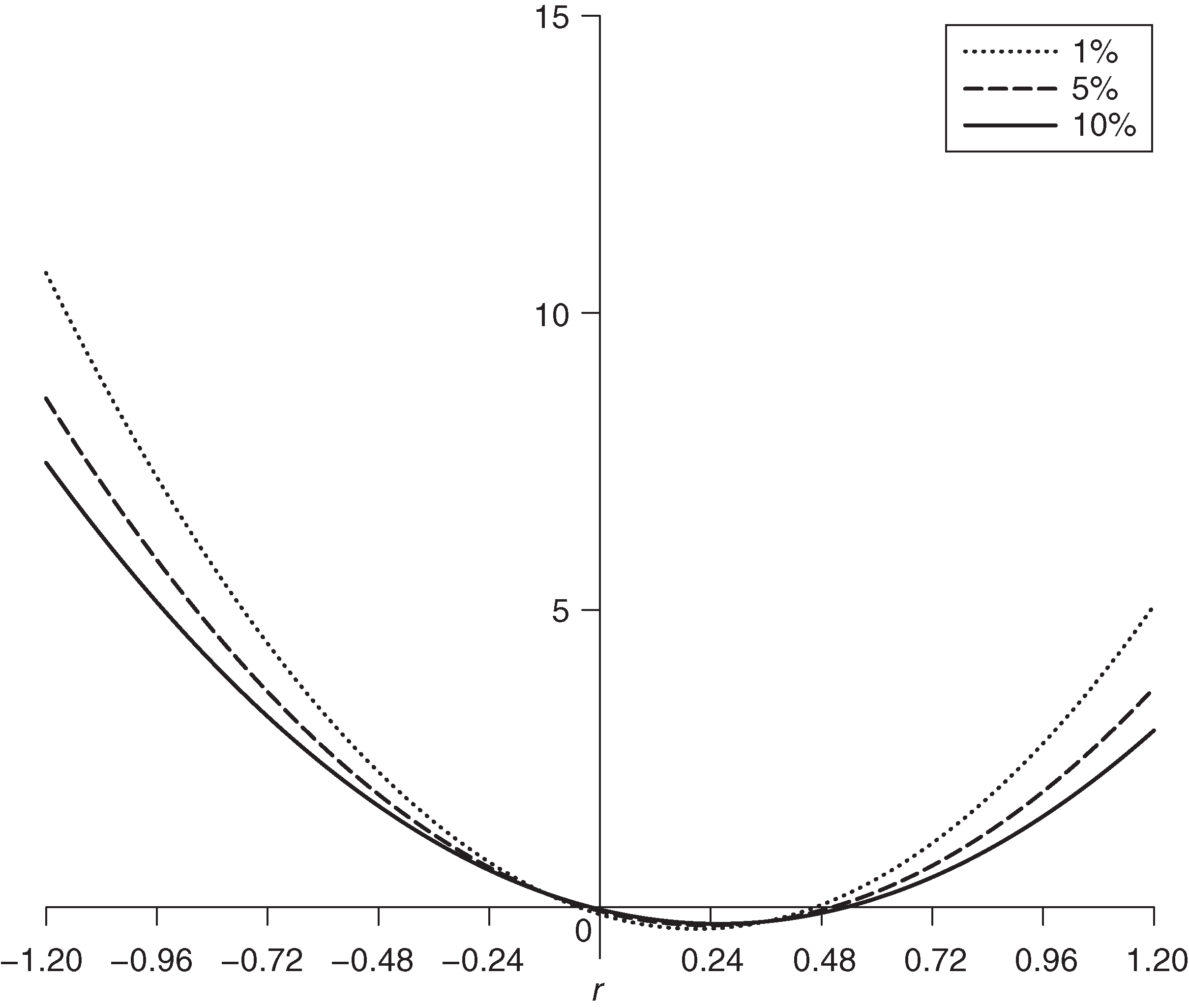
Figure 2 displays the normal distribution parametric influence function in terms of return $r$ for tail probabilities $\gamma =0.1,0.05,0.01$. It is striking how different these quadratic shapes are from the piecewise linear form of the nonparametric ES in Figure 1. One might argue that quadratic behavior is welcome for large negative returns. However, what is undesirable is quadratic behavior for positive returns, ie, large positive returns contribute to risk as measured by the normal distribution parametric risk estimator, and this is unwanted.

Figure 2: Parametric ES influence functions for normal distributions.

$t$-distribution ES MLE influence functions

The loglikelihood for the $t$-distribution for a single observed return $r$ is

	$l(v,s,\mu ;r)$	$=\mathrm{const}.-\ln s+\log \left(\mathrm{\Gamma }\left({\displaystyle \frac{\nu +1}{2}}\right)\right)-\log \left(\mathrm{\Gamma }\left({\displaystyle \frac{\nu }{2}}\right)\right)$
		$\mathrm{\hspace{1em}\hspace{1em}}-\frac{1}{2}\log (v)-{\displaystyle \frac{\nu +1}{2}}\ln \left(1+{\displaystyle \frac{1}{\nu }}{\left({\displaystyle \frac{r-\mu }{s}}\right)}^2\right).$		(5.12)

The score vector $?(r;?)=({\psi }_{\nu }(r;?),{\psi }_s(r;?),{\psi }_{\mu }(r;?))$ with $?={(\nu ,s,\mu )}^{\prime }$ is the derivative of the loglikelihood with respect to $?$, and it is straightforward to derive the form of the components ${\psi }_{\nu }$, ${\psi }_s$, ${\psi }_{\mu }$. The result in the convenient form used by Lucas (1997) is

$$\left[\begin{array}{c}\hfill {\psi }_{\nu }\hfill \\ \hfill {\psi }_s\hfill \\ \hfill {\psi }_{\mu }\hfill \end{array}\right]=\left[\begin{array}{c}\hfill \frac{1}{2}\left(\mathrm{\Omega }\left(\frac{v+1}{2}\right)-\mathrm{\Omega }\left(\frac{v}{2}\right)\right)-\frac{1}{2}\log \left(1+\frac{{(r-\mu )}^2}{v{s}^2}\right)+\frac{s}{2\nu }{\psi }_s(r)\hfill \\ \hfill {\psi }_s(r)\hfill \\ \hfill \frac{(v+1)(r-\mu )}{v{s}^2+{(r-\mu )}^2}\hfill \end{array}\right],$$

(5.13)

where

$${\psi }_s(r)=\frac{\nu }{s}\frac{{(r-\mu )}^2-s^2}{v{s}^2+{(r-\mu )}^2}$$

is the score function for scale and $\mathrm{\Omega }(\nu )=\mathrm{d}\log \mathrm{\Gamma }(\nu )/\mathrm{d}\nu$ is the di-gamma function.³³ 3 The sign difference in Lucas (1997) is due to the fact that he works with a loss function to be minimized rather than a likelihood to be maximized.

The score functions for location and scale are both bounded, but the score function ${\psi }_{\mu }(r;s,\mu )$ for location is redescending in the sense that it goes to $0$ as $r\to \pm \mathrm{\infty }$, while the score function ${\psi }_s(r;s,\mu )$ has the limiting positive value $\nu /s$ as $r\to \pm \mathrm{\infty }$. These behaviors of the score functions reflect the known robustness property of the $t$-distribution joint MLE of location and scale for the case of known degrees of freedom. However, the score function for degrees of freedom is logarithmically unbounded.

The information matrix for $?$ is

and straightforward but tedious integration shows that

(5.14)

where the derivative ${\mathrm{\Omega }}^{\prime }(\nu )$ is known as the tri-gamma function.⁴⁴ 4 This result may also be obtained, with a little effort, as a special case of the multivariate elliptical distribution results in Lange et al (1989). A simpler derivation for this univariate case was provided by Zhang and Green (2017). The above information matrix has the block-diagonal form

(5.15)

It can easily be verified that the upper-left two-by-two matrix is positive definite for $v>0$, ie, $AB>D^2$, and so the inverse of the information matrix exists and is given by

(5.16)

The block-diagonal form of (5.16) reveals that the $t$-distribution location MLE is (asymptotically) uncorrelated with the degrees of freedom and scale MLEs, but the latter two are correlated with each other to an extent determined by the parameter values $?={(\nu ,s,\mu )}^{\prime }$.

In our current notation, the $t$-distribution parametric ES measure is

$$\rho (?)={\rho }_{\mathrm{ES}}(\nu ,s,\mu )=-\mu +\frac{g_{\gamma ,\nu }}{\gamma }s,$$

(5.17)

where $g_{\gamma ,\nu }$ is given by (2.9), and the corresponding gradient vector is

$$\nabla {\rho }_{\mathrm{ES}}(\nu ,s,\mu )={(\frac{s}{\gamma }\frac{\partial g_{\gamma ,\nu }}{\partial \nu },\frac{g_{\gamma ,\nu }}{\gamma },-1)}^{\prime }.$$

(5.18)

When needed for computational purposes, we approximate the derivative of $g_{\gamma ,\nu }$ with respect to $\nu$ using the finite difference quotient

$$\frac{\partial g_{\gamma ,v}}{\partial \nu }\approx \frac{g_{\gamma ,v+\epsilon }-g_{\gamma ,v}}{\epsilon },\epsilon =0.001.$$

Plugging the above vector score function, information matrix inverse and gradient vector into (5.6) gives the $t$-distribution parametric ES influence function formula for unknown degrees of freedom:

$${\mathrm{IF}}_{\mathrm{ES}}(r;\mu ,s,\mu )=\nabla {\rho }_{\mathrm{ES}}(\nu ,s,\mu )\cdot {?}_{\nu ,s,\mu }^{-1}\cdot ?(r;?).$$

(5.19)

Figure 3 shows the influence function for the case $\nu =5$. This influence function is unbounded, but that it is only logarithmically unbounded follows from the fact that the score functions for location and scale in (5.13) are bounded. Thus, the ES estimator with unknown degrees of freedom is less influenced by outliers than the parametric normal distribution ES estimator that is unbounded in a quadratic manner.

Figure 3: $t$-distribution parametric ES influence functions.

In Appendix B (available online), we discuss $t$-distribution ES MLEs with known degrees of freedom and show that they have bounded influence functions.

6 Asymptotic variance of expected shortfall estimators

Under standard regularity conditions, a risk estimator ${\widehat{\rho }}_n$ that converges in probability to the true risk measure $\rho (F)$ also converges to a normal distribution

$$\sqrt{n}({\widehat{\rho }}_n-\rho (F))\stackrel{d}{\to }N(0,V_{\widehat{\rho }}),$$

(6.1)

where $V_{\widehat{\rho }}=V_{\widehat{\rho }}(F)$ is the estimator’s asymptotic variance. When $F$ is a parametric distribution $F_{?}$, we have $V_{\widehat{\rho }}=V_{\widehat{\rho }}(F_{?})=V_{\widehat{\rho }}(?)$.

Hampel (1974) showed that for iid returns the asymptotic variance is given by the expected value of the squared influence function at the distribution $F$:

$$V_{\widehat{\rho }}=E_F({\mathrm{IF}}_{\widehat{\rho }}^2(r;F))=\int {\mathrm{IF}}_{\widehat{\rho }}^2(r;F)dF(r).$$

(6.2)

The above result follows from the Filippova (1962) expansion

$$\sqrt{n}(\rho (F_n)-\rho (F))=\frac{1}{\sqrt{n}}\sum _{i=1}^n{\mathrm{IF}}_{\widehat{\rho }}(r_i;F)+\text{remainder},$$

(6.3)

where the remainder converges to zero in probability. For iid returns, the Hampel result is immediate once we take into account that, as Hampel noted, the influence function has zero expected value at distribution $F$.

In the next two subsections, we use the asymptotic variance formula (6.2) along with the influence function formulas derived in Sections 4–7 to compute and compare the large sample variances and standard errors of the nonparametric and parametric MLE ES estimators. Then, in Section 6.3, we discuss the computation of the ES estimator variance when the returns are no longer independent.

6.1 Asymptotic variance of nonparametric ES estimators

The following nonparametric form of the asymptotic variance formula for nonparametric ES is derived in Appendix A (available online):

$$V_{{\widehat{\mathrm{ES}}}_{\mathrm{NP}}}=\frac{1}{{\gamma }^2}{\int }_{-\mathrm{\infty }}^{q_{\gamma }}{r}^{2}dF(r)+\left(\frac{1}{\gamma }-1\right)q_{\gamma }^2-\left(2-\frac{2}{\gamma }\right){\mathrm{ES}}_{\gamma }{q}_{\gamma }-{\mathrm{ES}}_{\gamma }^2,$$

(6.4)

where $q_{\gamma }=q_{\gamma }(F)$ and ${\mathrm{ES}}_{\gamma }={\mathrm{ES}}_{\gamma }(F)$. Appendix A also shows that the above formula has the following forms for normal distributions and $t$-distributions.

Nonparametric ES estimator variance for normally distributed returns

$$V_{{\widehat{\mathrm{ES}}}_{\mathrm{NP}},\mathrm{N}}={\sigma }^2\left[\left(\frac{1}{\gamma }+\frac{z_{\gamma }^2}{\gamma }-z_{\gamma }^2\right)+\frac{(1-2\gamma )z_{\gamma }}{{\gamma }^2}\varphi (z_{\gamma })-\frac{1}{{\gamma }^2}{\varphi }^2(z_{\gamma })\right].$$

(6.5)

Nonparametric ES estimator variance for $t$-distributed returns

$$V_{{\widehat{\mathrm{ES}}}_{\mathrm{NP},t\text{-dist}}}=\frac{s^2}{{\gamma }^2}[(1-2\gamma )md{q}_{\gamma ,v}+m^{2}p+(\gamma -{\gamma }^2)q_{\gamma ,v}^2-m^2{d}^2],$$

(6.6)

where

(6.7)

Figure 4 shows the asymptotic standard error, ie, the square root of the asymptotic variance, of a nonparametric ES estimator versus tail probability $\gamma$ for degrees of freedom three, five, seven and infinity, the latter being the normal distribution. The fatter the tail (the smaller the degree of freedom), the more rapidly the ES estimator variance and standard error increases for small tail probabilities.

Risk managers often want to choose a small tail probability to measure the extreme loss risk, but careful attention should be paid to the trade-off between the choice of tail probability and the choice of risk estimator variability; this is especially the case for $t$-distributions. Using the asymptotic variance formula, we find that for a (without loss of generality) standard normal distribution, a nonparametric ES estimator has asymptotic standard errors $\mathrm{SE}({\mathrm{ES}}_{0.025})=0.413$ and $\mathrm{SE}({\mathrm{ES}}_{0.01})=0.592$ for tail probabilities of 2.5% and 1%, respectively. In this case, one might not find the reduction in standard error of about 30% when going from a 1% tail probability to a BIS-recommended 2.5% of great concern. However, for the case of a standard $t$-distribution with three degrees of freedom, those two standard errors change to $\mathrm{SE}({\mathrm{ES}}_{0.025})=2.949$ and $\mathrm{SE}({\mathrm{ES}}_{0.01})=6.266$, and the reduction in standard error when going from a 1% tail probability to a 2.5% tail probability is 53%. The Basel III recommendation is attractive in this regard.

Figure 4: Nonparametric ES estimator standard error under $t$-distributions.

6.2 Asymptotic variance of ES MLEs

The derivation of the variance formulas for ES MLEs is considerably simpler than in the nonparametric case. Using (5.6) in (6.2), we have the following general variance expression for an ES MLE:

	$V_{{\widehat{\mathrm{ES}}}_{\mathrm{MLE}}}$	$=E_F[{\mathrm{IF}}_{\mathrm{par}}^2(r;\widehat{\rho },F)]$
		$=E_F[\nabla \rho {(?)}^{\prime }\cdot {?}_{?}^{-1}\cdot ?(r;?){?}^{\prime }(r;?)\cdot {?}_{?}^{-1}\cdot \nabla \rho (?)]$
		$=\nabla \rho {(?)}^{\prime }\cdot {?}_{?}^{-1}\cdot \nabla \rho (?).$		(6.8)

Plugging the normal distribution formulas (5.8) and (5.10) into (6.8) gives the expression for the variance of ES MLEs for normal distributions:

$$V_{{\widehat{\mathrm{ES}}}_{\text{MLE–N}}}={\sigma }^2\left(1+\frac{{\varphi }^2(z_{\gamma })}{2{\gamma }^2}\right).$$

(6.9)

Plugging the $t$-distribution with unknown degrees of freedom formulas (5.16) and (5.18) into (6.8) gives the expression for the variance of ES MLEs for $t$-distributions:

$$V_{{\widehat{\mathrm{ES}}}_{\text{MLE–T}}}=\nabla {\rho }_{\mathrm{ES}}{(\nu ,s,\mu )}^{\prime }\cdot {?}_{\nu ,s,\mu }^{-1}\cdot \nabla {\rho }_{\mathrm{ES}}(\nu ,s,\mu ).$$

(6.10)

Figure 5 shows the large sample standard errors of $t$-distribution parametric ES MLE with unknown degrees of freedom when the true degrees of freedom are three, six and infinity (the normal distribution). The results should be compared with those of the nonparametric ES estimators in Figure 4. The standard errors of Figure 4 are larger than those of Figure 5, and more so for the smaller tail probabilities. This is to be expected since an ES MLE has the smallest attainable large sample variance and standard error.

Figure 5: Parametric $t$-distribution ES MLE standard error.

Inefficiency of the nonparametric ES estimator

Since our parametric ES estimators are MLEs, they achieve the minimum possible asymptotic variance. Correspondingly, a nonparametric ES estimator at a given return distribution has an asymptotic variance that is bounded below by the asymptotic variance of the parametric ES estimator for that distribution. It is common practice to define the efficiency of an estimator other than the MLE as the ratio of the variance of the MLE to the variance of the alternative estimator, and to express this ratio in percentage terms. Since standard deviation is a more natural comparison scale than variance, we define the efficiency of a nonparametric ES estimator at a given return distribution as the ratio of the asymptotic standard deviation of the ES MLE for that distribution to the asymptotic standard deviation of the nonparametric ES estimator for that distribution. The usual definition of efficiency in terms of ratios of variances is obtained from our standard deviation-based ratios by squaring the latter.

Table 2 displays the standard error efficiencies (rounded to the nearest integer) of nonparametric ES estimators for normally distributed returns and tail probabilities 1%, 2.5%, 5% and 50%. Not surprisingly, the efficiency of the nonparametric ES estimator decreases with decreasing tail probability.

Table 2: Nonparametric ES estimator efficiency for normally distributed returns.

	Tail probability
	0.01	0.025	0.05	0.5
Efficiency (%)	46	60	72	98

Table 3: Nonparametric ES estimator efficiency for $t$-distributed returns.

	Tail probability
	0.01	0.025	0.05	0.5
Efficiency (%) with $\text{DOF}=\text{3}$	50	59	64	81
Efficiency (%) with $\text{DOF}=\text{5}$	62	69	72	92
Efficiency (%) with $\text{DOF}=\text{7}$	65	71	73	96

Table 3 displays the standard error efficiencies (rounded to the nearest integer) of nonparametric ES estimators for $t$-distributed returns with $\text{DOF}=3,5,7$.

6.3 Asymptotic variance of ES estimators when returns are not independent

If a risk manager is concerned that the returns have neither a normal nor a $t$-distribution, there is still the possibility of using the nonparametric variance expression (6.3). However, if the assumption of iid returns is not satisfied, then none of the previous formulas in this section are valid. Here, we briefly discuss the situation where the returns are not independent but are identically distributed, ie, the returns are a stationary random process.

Two possibilities need to be considered. The first is that the returns are serially correlated. The second is that the returns are those of a GARCH process, whereby they are uncorrelated but not independent. In both of the above cases, the identically distributed series ${\mathrm{IF}}_{\widehat{\rho }}(r_i;F)$, $i=1,2,\mathrm{\dots },n$, will be serially correlated, not only for ES but also for other risk and performance measures.⁵⁵ 5 In the case of GARCH processes, the serial correlation of the influence function transformed returns series is, of course, obvious for volatility estimates. However, it also occurs for most risk and performance estimators because their influence functions are nonlinear transformations of the returns. In this case, the problem of estimating the variance of a risk or performance estimator reduces to that of estimating the variance of a sum of serially correlated random variables, ie, the standardized sum of influence functions in (6.3).

The conventional solution to correcting for serial correlation in the context of econometric time series models is to use a Newey–West-type correction based on a summation of kernel weighted lag-$k$ covariance estimates, where the kernel weights are $0$ outside a prescribed bandwidth that grows with sample size (see, for example, Newey and West 1987, 1994). However, there is an alternative frequency domain approach to this problem, which is based on the fact that, for a stationary process, the large-sample variance of a serially correlated sum of random variables is equal to the spectral density function evaluated at zero frequency. A method of computing standard errors of sums of correlated stationary time series random variables by estimating a spectral density at zero frequency was proposed and shown to work reasonably well by Heidelberger and Welch (1981).

That initial spectral density approach was improved upon by Chen and Martin (2019), who used a special method of estimating the spectral density at the origin of the influence function transformed series appearing in (6.3). This method involves using a generalized linear model (GLM) for fitting polynomials to exponentially distributed periodogram values, with elastic net (L1 and L2) regularization. It was evaluated for a number of risk and performance estimators (including ES), for serially correlated hedge fund returns and for simulated $\mathrm{AR}(1)$ returns, where it was shown to provide better standard error estimates than Newey–West methods. Simulation studies also showed that the method works quite well for $\mathrm{GARCH}(1,1)$ returns.

7 Finite sample standard error approximation performance

The closed-form formulas of the ES asymptotic variances in Section 8 allow us to compute finite sample standard error approximations by plugging in the estimates of unknown parameters, taking the square root of the resulting expression and dividing by the square root of the sample size. However, the resulting standard error is subject to an approximation error that one anticipates will increase as the sample size, tail probability and degrees of freedom decrease. In order to evaluate how accurate such approximations are for nonparametric versus parametric ES, we use a Monte Carlo simulation to estimate “true” finite sample standard errors, against which we evaluate finite sample standard errors. Henceforth, we refer to the former as SEmc and to the latter as simply “standard error”.

The Monte Carlo study includes both normal and $t$-distributed return distributions, and by location and scale equivariance of ES it suffices to study the standard errors for standard normal and standard $t$-distributions. Our study uses sample sizes $N=60,100,200,400$, tail probabilities 1%, 2.5% and 5%, and $t$-distributions $\text{DOF}=3,5,10$. The steps for estimating the SEmc of an ES estimator $\widehat{\mathrm{ES}}$ are as follows.

1. (1)

   Simulate a sample of size $N$ from the return distribution $F$.

2. (2)

   Compute the risk estimate ${\widehat{\mathrm{ES}}}_1$ (parametric and nonparametric) for a sample of size $N$.

3. (3)

   Repeat (1) and (2) $M$ times and denote the estimates as ${\widehat{\mathrm{ES}}}_1,{\widehat{\mathrm{ES}}}_2,\mathrm{\dots },{\widehat{\mathrm{ES}}}_M$.

4. (4)

   Calculate SEmc as the sample standard deviation of ${\widehat{\mathrm{ES}}}_1,{\widehat{\mathrm{ES}}}_2,\mathrm{\dots },{\widehat{\mathrm{ES}}}_M$.

All of the following results are based on $M=1000$ Monte Carlo replications.

Computation of nonparametric ES estimators and parametric ES MLEs

Nonparametric ES estimators are computed using (2.12); approximations are described in the next subsection for two cases with tail probability 2.5%, where the product of $n$ and $p$ is not an integer.

Parametric ES MLEs for $t$-distributions are computed using the formulas in Table 1 with MLEs as the parameter estimators.

As for parametric (MLE) ES estimators, we compute parametric $t$-distribution ES estimator MLEs with the view that they will provide high degrees of freedom approximations to parametric normal distribution ES estimator MLEs if the returns are actually normally distributed. Also, in view of the closeness of the asymptotic standard errors of normal distribution parametric ES and those of the SSD variant in (9.9) and (9.10), displayed in Figure 10, we do not bother with that SSD variant in this Monte Carlo study.

Standard error approximations for nonparametric ES estimators

A natural way to estimate the asymptotic variance of a nonparametric ES estimator is to use the nonparametric asymptotic variance expression (6.4). When $n=60$ and $n=100$ at tail probability $p=0.01$, we have $\lceil \mathrm{NP}\rceil =1$, $q_{\gamma }=-r_{(1)}$ and ${\mathrm{ES}}_{\gamma }=-r_{(1)}$. In this case, (4.2) gives ${\mathrm{IF}}_{\mathrm{ES}}(r;F)=0$ for all values of $r$ and the asymptotic variance formula (6.2) does not give a meaningful standard error estimate. This also means that one cannot obtain a meaningful standard error estimate using the empirical version of (6.2), ie, the sample average of the squared values of the influence function evaluated at the observed data. There are just two cases in our Monte Carlo study where $\mathrm{NP}$ is not integer valued, namely $n=60$ and $n=100$ at tail probability $p=0.025$. For these cases, we use natural averages of order statistics to compute estimates of $q_{\gamma }$ and ${\mathrm{ES}}_{\gamma }$.⁶⁶ 6 For $p=0.025$, we used $q_{\gamma }=-(r_{(1)}+r_{(2)})/2$ and ${\mathrm{ES}}_{\gamma }=-(r_{(1)}+(r_{(1)}+r_{(2)})/2)/2$ for $n=60$, and $q_{\gamma }=-(r_{(2)}+r_{(3)})/2$ and ${\mathrm{ES}}_{\gamma }=-[(r_{(1)}+r_{(2)})/2+(r_{(1)}+r_{(2)}+r_{(3)})/3]/2$ for $n=100$.

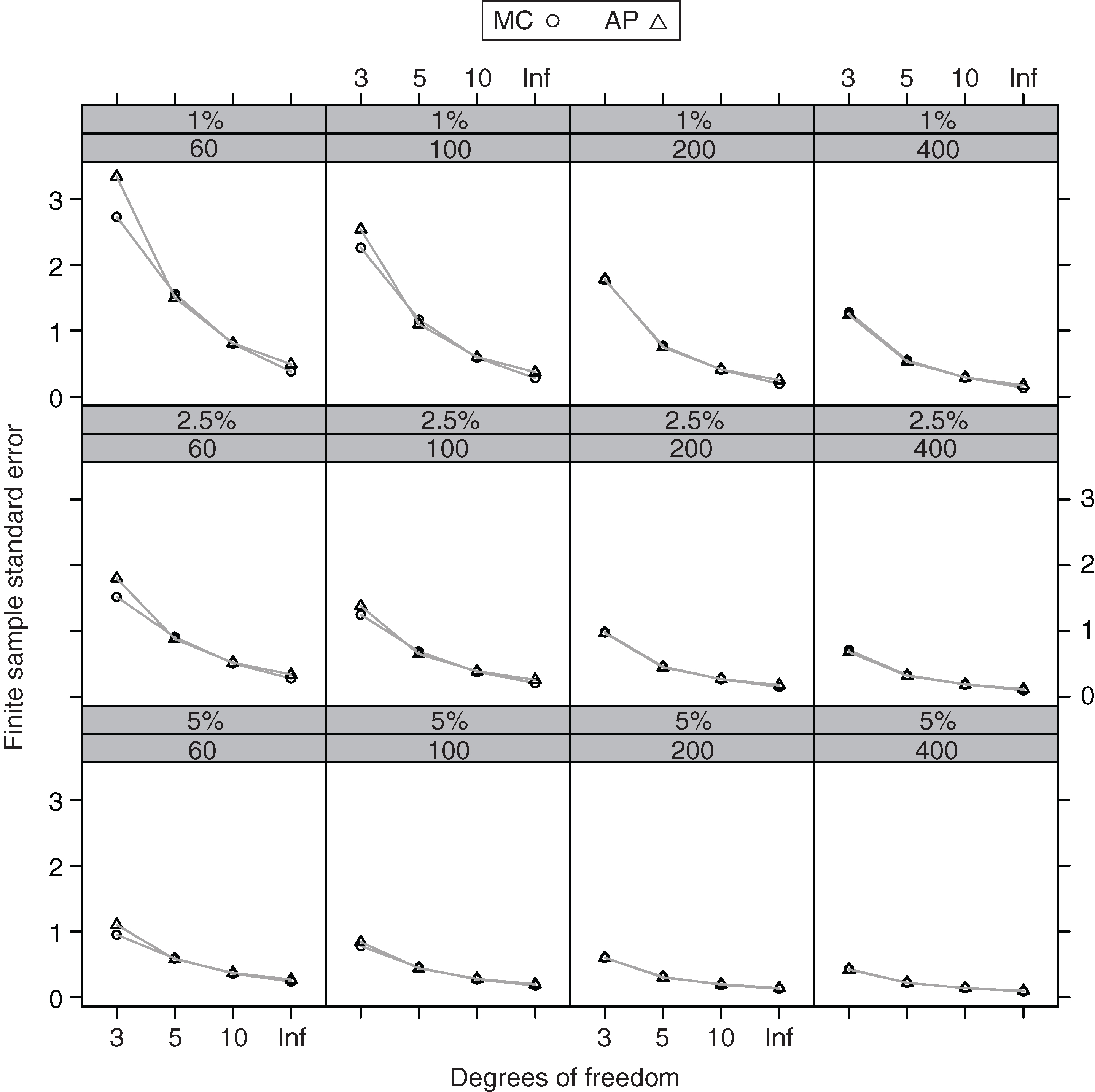
The results are displayed in Table 4 and Figure 6, where SEap indicates the finite sample approximate standard error results, RE is the percent relative error and $\text{DOF}=\text{Inf}$ indicates that the return replicates were generated according to a standard normal distribution. The NAs are for cases in which (6.2) does not yield a meaningful standard error estimate. We see that all of the finite sample standard error approximations SEap are underestimates of the Monte Carlo SEmc values, with absolute percent errors in double digits, except for $p=0.05$: this has one case at $n=200$ and three cases at $n=400$.

Table 4: Standard error approximation for nonparametric ES estimator.

		Sample size $?$
		60			100			200			400
Tail	DOF	SEmc	SEap	RE	SEmc	SEap	RE	SEmc	SEap	RE	SEmc	SEap	RE
0.01	0 3	3.27	NA	NA	4.10	NA	NA	3.09	1.40	$-$55%	2.18	1.46	$-$33%
	0 5	1.33	NA	NA	1.45	NA	NA	1.11	0.55	$-$50%	0.79	0.60	$-$25%
	10	0.72	NA	NA	0.72	NA	NA	0.53	0.29	$-$45%	0.42	0.31	$-$25%
	Inf	0.45	NA	NA	0.42	NA	NA	0.31	0.16	$-$48%	0.23	0.17	$-$27%
0.025	0 3	2.65	0.63	$-$76%	2.20	1.06	$-$52%	1.54	1.06	$-$31%	1.10	0.86	$-$22%
	0 5	1.11	0.31	$-$72%	0.88	0.50	$-$42%	0.65	0.48	$-$26%	0.46	0.40	$-$13%
	10	0.62	0.19	$-$70%	0.49	0.30	$-$38%	0.35	0.29	$-$18%	0.27	0.23	$-$12%
	Inf	0.40	0.13	$-$68%	0.31	0.19	$-$38%	0.23	0.18	$-$21%	0.16	0.14	$-$13%
0.05	0 3	1.51	0.91	$-$40%	1.25	0.86	$-$31%	0.90	0.71	$-$21%	0.65	0.54	$-$16%
	0 5	0.73	0.47	$-$35%	0.58	0.45	$-$22%	0.42	0.36	$-$15%	0.30	0.28	0 $-$7%
	10	0.45	0.31	$-$31%	0.35	0.29	$-$16%	0.25	0.23	0 $-$9%	0.19	0.18	0 $-$7%
	Inf	0.31	0.21	$-$30%	0.24	0.20	$-$17%	0.18	0.16	$-$13%	0.13	0.12	0 $-$9%

Figure 6: Nonparametric standard error approximation for nonparametric ES estimator.

Standard error approximations for $t$-distribution ES MLEs

When using $t$-distribution ES estimator MLEs, a risk manager is trusting that the $t$-distribution family offers a sufficiently good assumption for risk management purposes, and in that case there is little motivation to consider a nonparametric standard error estimator. Thus, (6.10) is again used, with the parameter MLEs having already been computed when computing the ES.

Table 5 and Figure 7 show results for the standard error approximations of $t$-distribution ES MLEs. As anticipated, except for $p=0.01$ and $n=60$, the Monte Carlo values SEmc in Table 5 are uniformly smaller than those in Table 4: often considerably so. Further, the relative error values are much smaller, except for in the normal distribution case $\text{DOF}=\text{Inf}$, where the large relative error values are due to the high variability of the $t$-distribution DOF estimator for normally distributed returns. Nonetheless, the absolute values of SEap are uniformly smallest for $\text{DOF}=\text{Inf}$.

Table 5: Standard error approximation for parametric $t$-distribution ES MLE.

		Sample size $?$
		60			100			200			400
Tail	DOF	SEmc	SEap	RE	SEmc	SEap	RE	SEmc	SEap	RE	SEmc	SEap	RE
0.01	0 3	2.73	3.34	23%	2.26	2.54	12%	1.77	1.78	0 0%	1.28	1.24	0 $-$4%
	0 5	1.56	1.50	0 $-$4%	1.17	1.10	0 $-$7%	0.77	0.75	0 $-$2%	0.55	0.53	0 $-$4%
	10	0.80	0.81	0 1%	0.59	0.60	0 2%	0.41	0.41	0 0%	0.29	0.29	0 0%
	Inf	0.38	0.49	29%	0.28	0.37	33%	0.19	0.25	33%	0.13	0.17	33%
0.025	0 3	1.52	1.80	19%	1.25	1.38	10%	0.98	0.97	0 0%	0.71	0.68	0 $-$4%
	0 5	0.91	0.88	0 $-$3%	0.69	0.65	0 $-$5%	0.46	0.45	0 $-$2%	0.33	0.32	0 $-$3%
	10	0.51	0.52	0 3%	0.38	0.39	0 3%	0.27	0.27	0 1%	0.19	0.19	0 1%
	Inf	0.28	0.34	21%	0.21	0.26	22%	0.15	0.18	19%	0.10	0.12	19%
0.05	3	0.95	1.10	16%	0.78	0.84	0 8%	0.60	0.60	0 0%	0.43	0.42	0 $-$4%
	5	0.59	0.58	0 $-$1%	0.45	0.44	0 $-$4%	0.31	0.30	0 $-$1%	0.22	0.22	0 $-$1%
	10	0.36	0.37	0 2%	0.27	0.28	0 3%	0.19	0.20	0 2%	0.14	0.14	0 2%
	Inf	0.24	0.27	12%	0.18	0.20	13%	0.13	0.14	0 9%	0.09	0.10	10%

Figure 7: Standard error approximation for parametric $t$-distribution ES estimator.

Relative efficiencies of nonparametric versus parametric ES estimators

Table 6 displays the Monte Carlo values of the ES MLE standard errors (SEmles) and the nonparametric ES standard errors (SEnps) along with the efficiencies of the nonparametric ES (Eff), defined as the ratio of SEmle to SEnp. Note that the finite sample efficiency of 57% in Table 6, with tail probability 2.5%, $\text{DOF}=\text{Inf}$ and a sample size of 400, compares well with the asymptotic efficiency of 60.4% given in Table 2 for normal distributions.

Table 6: Efficiency of nonparametric standard error versus parametric standard error.

		Sample size $?$
		60			100			200			400
Tail	DOF	SEmle	SEnp	Eff	SEmle	SEnp	Eff	SEmle	SEnp	Eff	SEmle	SEnp	Eff
0.01	0 3	2.73	3.27	83%	2.26	4.10	55%	1.77	3.09	57%	1.28	2.18	59%
	0 5	1.56	1.33	117%	1.17	1.45	81%	0.77	1.11	69%	0.55	0.79	70%
	10	0.80	0.72	110%	0.59	0.72	82%	0.41	0.53	76%	0.29	0.42	69%
	Inf	0.38	0.45	85%	0.28	0.42	66%	0.19	0.31	60%	0.13	0.23	57%
0.025	0 3	1.52	2.65	57%	1.25	2.20	57%	0.98	1.54	63%	0.71	1.10	64%
	0 5	0.91	1.11	82%	0.69	0.88	79%	0.46	0.65	71%	0.33	0.46	72%
	10	0.51	0.62	81%	0.38	0.49	78%	0.27	0.35	76%	0.19	0.27	71%
	Inf	0.28	0.40	72%	0.21	0.31	70%	0.15	0.23	66%	0.10	0.16	64%
0.05	0 3	0.95	1.51	63%	0.78	1.25	62%	0.60	0.90	67%	0.43	0.65	67%
	0 5	0.59	0.73	81%	0.45	0.58	79%	0.31	0.42	72%	0.22	0.30	73%
	10	0.36	0.45	81%	0.27	0.35	78%	0.19	0.25	76%	0.14	0.19	72%
	Inf	0.24	0.31	78%	0.18	0.24	76%	0.13	0.18	73%	0.09	0.13	71%

Summary of Monte Carlo results

The standard error estimator for nonparametric ES consistently underestimates the Monte Carlo estimates of the true standard error, very substantially. A risk manager is likely to be reluctant to use nonparametric ES with sample sizes of less than 400 at Basel III’s recommended 2.5% tail probability; they would perhaps use our empirical results to create rules of thumb for the upward adjustment of calculated approximate standard error estimates.

The standard error estimator for the ES $t$-distribution MLE is remarkably good for a sample size of 200 or above for all three tail probabilities and all degrees of freedom: that is, except for the double-digit percent overestimation for the normal distribution case $\text{DOF}=\text{Inf}$, where nonetheless the standard error estimates are very small.

For 2.5% and 5% tail probabilities at sample sizes of 200 and 400, the standard error efficiency of the nonparametric ES estimators, relative to that of the $t$-distribution ES MLE, ranges from 63% to 76%. It should be noted that, except for in the $\text{DOF}=3$ cases, the standard error efficiencies of nonparametric ES estimators at sample sizes of 60, 100 and 200 are almost always higher than for a sample size of 400.

8 Influence function sufficient condition for the coherence monotonicity axiom

Recall that a risk measure $\rho (R)=\rho (F)$ based on a random return $R$ with distribution $F$ is said to be coherent if it satisfies the following four axioms.

Translation equivariance ($\mathrm{TE}$):

$\rho (R+b)=\rho (R)-b$ for any constant $b$.

Positive homogeneity ($\mathrm{PH}$):

$\rho (\lambda R)=\lambda \rho (R)$ for any $\lambda \ge 0$.

Subadditivity ($\mathrm{SUB}$):

$\rho (R_1+R_2)\le \rho (R_1)+\rho (R_2)$.

Monotonicity ($\mathrm{MO}$):

$R\ge 0$ with probability $1\Rightarrow$ $\rho (R)\le 0$ or, equivalently, $R_1\ge R_2$ with probability $1\Rightarrow$ $\rho (R_1)\le \rho (R_2)$.

Lack of coherence of normal distribution parametric ES

It turns out, perhaps surprisingly to many, that the normal distribution ES risk measure (2.5) lacks coherence. This follows as a special case of a more general result stated by Scandolo (2015) for any mean–standard deviation (mean–SD) risk measure of the form

(8.1)

Namely, $\rho (F)$ satisfies the PH, SUB and TE axioms but not the MO axiom. To prove that the above risk measure does not satisfy the MO axiom, we just need to check Scandolo’s suggestion that it can be shown by using a discrete random variable that takes on two values. For example, let $F$ be the discrete distribution

of a nonnegative random variable, and note that we will have $\rho (R)=\rho (F)>0$ provided that $\sigma (F)/\mu (F)>1/a$. Then, since

$$\frac{\sigma (F)}{\mu (F)}={\left[(1-k^{-1})+\frac{{(k-1)}^2}{k}\right]}^{1/2}={[k-1]}^{1/2},$$

we see that for any $a>0$ the above expression can be made larger than $a^{-1}$. Thus, (8.1) fails to satisfy the MO property.

Lack of coherence of $t$-distribution ES MLE

In the case of a $t$-distribution, the scale functional $s(F)$ is symmetric, as is its MLE. Thus, we conjecture that the $t$-distribution ES MLE fails to be coherent, but we do not yet have proof of this.

Monotonicity of a parametric risk measure influence function and coherence

The failure of (8.1) to satisfy the MO property is associated with the symmetric nature of the standard deviation functional for any symmetric location and scale family, which, in turn, is responsible for the roughly symmetric behavior of the ES normal distribution MLE influence function (5.11). On the other hand, the monotonicity of a risk measure estimator as exemplified by the nonparametric ES estimator displayed in Figure 1(b) is intuitively very appealing. One therefore wonders if there is a connection between the monotonicity of a risk measure estimator influence function and the MO property of a risk measure. The following lemma shows that there is indeed a very general connection.

Lemma 8.1.

If there exists an estimator ${\widehat{\rho }}_n$ of a parametric risk measure functional $\rho \mathit{}\mathrm{(}?\mathit{}\mathrm{(}F\mathrm{)}\mathrm{;}{F}_{?}\mathrm{)}$ whose influence function ${\mathrm{IF}}_{\widehat{\rho }}\mathit{}\mathrm{(}r\mathrm{;}F\mathrm{)}$ is monotone decreasing, and if the risk measure $\rho \mathit{}\mathrm{(}?\mathit{}\mathrm{(}{F}_p\mathrm{)}\mathrm{;}{F}_{?}\mathrm{)}$ is continuous in $p$ at $p\mathrm{=}\mathrm{0}$, then the risk measure satisfies the MO coherence axiom.

Proof.

First, we express the risk measure as $\tilde{\rho }(F)=\tilde{\rho }(F;F_{?})=\rho (?(F);F_{?})$, keeping in mind that the analytic form of $\tilde{\rho }(\cdot )$ is determined by the assumed distribution family $F_{?}$. We let $F=F_p$ as given by (3.1). We note that the mixture distribution $F_p$ used in the definition of influence function formula (3.2) depends on a return value $r$, which we take to be the realization of a random return $R$. We make this explicit by writing $\tilde{\rho }(F_p)=\tilde{\rho }(R;F_p)$ and note that, according to (3.2), we have

$$\tilde{\rho }(R;F_p)=\tilde{\rho }(F_0)+p\cdot {\mathrm{IF}}_{\widehat{\rho }}(R;F_0)+o(p).$$

If with probability $1$ we have $R_1>R_2$, then for  we have, with probability $1$, that

	$\tilde{\rho }(R_1;F_p)-\tilde{\rho }(R_2;F_p)$	$=p[{\mathrm{IF}}_{\widehat{\rho }}(R_1;F_0)-{\mathrm{IF}}_{\widehat{\rho }}(R_2;F_0)]+o(p)$
		$\le p\cdot 0+o(p)$
		$=o(p),$

and within the limit $p\to 0$ we have $\tilde{\rho }(R_1,F_0)\le \tilde{\rho }(R_2,F_0)$. ∎

Note However, the continuity of $\tilde{\rho }(F_p)=\tilde{\rho }(r;F_p)=\rho (?(F_p);F_{?})$ in $p$ at $p=0$ for the special mixture model (3.1) is easily proved for the normal distribution parametric risk measure (2.3) by proving that the mean and volatility functionals $\mu (F_p)$ and $\sigma (F_p)$ are continuous in $p$ at $p=0$.⁷⁷ 7 This is a much weaker kind of continuity than the continuity of a parameter functional in the usual metrics used in robustness, eg, the Lévy–Prokhorov metric, for which the mean and volatility functionals are not continuous.

9 Mean–semi-standard deviation risk measure

In the previous section, it was shown that the normal distribution parametric ES measure fails to be coherent because it is a special case of the general class of mean–SD risk measures, all of which fail to be coherent due to lacking the MO property. From an influence function perspective, this is hardly surprising in view of the roughly symmetric nature of the normal distribution parametric ES risk measure influence function (and also that of a $t$-distribution), which results in a large positive return making a large contribution to risk. It is therefore natural to consider mean–SSD risk measures of the form

$${\mathrm{ES}}_{\mathrm{SSD}}(F)=-\mu (F)+a{\sigma }_{\mathrm{SSD}}(F)$$

(9.1)

for various positive values of the constant $a$ as alternatives to the normal distribution parametric risk measures (2.5). With the mean–SSD risk measure, we expect that large positive returns will not contribute much to risk.

As was pointed out by Scandolo (2015), the class of mean–SSD risk measures was studied some time ago by Fischer (2003), who showed that the risk measure (9.1) is coherent for . We note that this is a sufficient but not necessary condition on $a$. We now explore what values this constant takes on for the case of an SSD modification of normal distribution parametric ES.

Mean–SSD modification of normal distribution parametric ES

The functional form of SSD is

$${\sigma }_{\mathrm{SSD}}={\sigma }_{\mathrm{SSD}}(F)={\left({\int }_{-\mathrm{\infty }}^{\mu (F)}{(r-\mu (F))}^{2}dF(r)\right)}^{1/2},$$

(9.2)

and we will assume unless otherwise stated that the return distribution $F$ is symmetric about its mean. In that case, semi-variance ${\sigma }_{\mathrm{SSD}}^2$ has half the value of variance ${\sigma }^2$, and with $\sqrt{2}{\sigma }_{\mathrm{SSD}}$ replacing $\sigma$ in (2.5) we have the mean–SSD ES functional

$${\mathrm{ES}}_{\mathrm{SSD}}(\mu (F),{\sigma }_{\mathrm{SSD}}(F))=-\mu (F)+\frac{\varphi (z_{\gamma })}{\gamma }\sqrt{2}{\sigma }_{\mathrm{SSD}}(F);$$

(9.3)

this has the same value as normal distribution parametric ES (2.5). It should be noted that (9.3) is of the form (9.1), with

$$a_{\gamma }=\sqrt{2}\frac{\varphi (z_{\gamma })}{\gamma }.$$

(9.4)

Further, consistent estimators of $\mu (F)$ and ${\sigma }_{\mathrm{SSD}}(F)$ in (9.3) will result in a consistent (but inefficient) estimator of normal distribution parametric ES. The natural estimator ${\widehat{\mathrm{ES}}}_{\mathrm{SSD}}$ of ${\mathrm{ES}}_{\mathrm{SSD}}$ uses the sample mean $\widehat{\mu }$ and the sample SSD ${\widehat{\sigma }}_{\mathrm{SSD}}$⁸⁸ 8 The sample SSD is ${\widehat{\sigma }}_{\mathrm{SSD}}={((1/n){\sum }_{i=1}^n{[{(\widehat{\mu }-r_i)}^{+}]}^2)}^{1/2}$.

$${\widehat{\mathrm{ES}}}_{\mathrm{SSD}}=-\widehat{\mu }+\frac{\varphi (z_{\gamma })}{\gamma }\sqrt{2}{\widehat{\sigma }}_{\mathrm{SSD}}.$$

(9.5)

Influence function of the mean–SSD ES estimator

Since (9.3) is a linear combination of the mean functional and the SSD functional, the influence function of the SSD-based ES estimator is the corresponding linear combination of the influence functions for the sample mean and the SSD estimators:

	${\mathrm{IF}}_{{\widehat{\mathrm{ES}}}_{\mathrm{SSD}}}(r;F)$	$=-{\mathrm{IF}}_{\widehat{\mu }}(r;F)+{\displaystyle \frac{\varphi (z_{\gamma })}{\gamma }}\sqrt{2}{\mathrm{IF}}_{{\widehat{\sigma }}_{\mathrm{SSD}}}(r;F)$
		$=-(r-\mu )+{\displaystyle \frac{\varphi (z_{\gamma })}{\gamma }}\sqrt{2}{\mathrm{IF}}_{{\widehat{\sigma }}_{\mathrm{SSD}}}(r;F).$		(9.6)

Appendix C in the online version of this paper shows that

$${\mathrm{IF}}_{{\widehat{\sigma }}_{\mathrm{SSD}}}(r;F)=\frac{{(r-\mu )}^2{I}_{(-\mathrm{\infty },\mu ]}+2{\int }_{-\mathrm{\infty }}^{\mu }(\mu -x)dF(x)(r-\mu )-{\sigma }_{\mathrm{SSD}}^2}{2{\sigma }_{\mathrm{SSD}}},$$

and since ${\sigma }^2=2{\sigma }_{\mathrm{SSD}}^2$ we write the above expression as

$${\mathrm{IF}}_{{\widehat{\sigma }}_{\mathrm{SSD}}}(r;F)=\frac{{(r-\mu )}^2{I}_{(-\mathrm{\infty },\mu ]}+2{\int }_{-\mathrm{\infty }}^{\mu }(\mu -x)d{F}_0(x)(r-\mu )-{\sigma }_{\mathrm{SSD}}^2}{\sqrt{2}\sigma }-\frac{\sigma }{2\sqrt{2}}.$$

Substituting this into (9.4) gives

	${\mathrm{IF}}_{{\widehat{\mathrm{ES}}}_{\mathrm{SSD}}}(r;F)$	$={\displaystyle \frac{\varphi (z_{\gamma })}{\gamma \sigma }}{(r-\mu )}^2{I}_{(-\mathrm{\infty },\mu ]}(r)$
		$\mathrm{\hspace{1em}\hspace{1em}}+\left({\displaystyle \frac{\varphi (z_{\gamma })}{\gamma \sigma }}2{\displaystyle {\int }_{-\mathrm{\infty }}^{\mu }}(\mu -x)dF(x)-1\right)(r-\mu )-{\displaystyle \frac{\sigma \varphi (z_{\gamma })}{2\gamma }}.$		(9.7)

Note that the above influence function will be monotonic decreasing only if the coefficient of the linear term is nonpositive.

When the returns have a normal distribution $F=N(\mu ,{\sigma }^2)$, evaluation of the integral in the linear term above gives

$${\mathrm{IF}}_{{\widehat{\mathrm{ES}}}_{\mathrm{SSD}}}(r;F)=\frac{\varphi (z_{\gamma })}{\gamma \sigma }{(r-\mu )}^2{I}_{(-\mathrm{\infty },\mu ]}(r)+\left(\sqrt{2}\frac{\varphi (z_{\gamma })}{\gamma }\sqrt{\frac{1}{\pi }}-1\right)(r-\mu )-\frac{\sigma \varphi (z_{\gamma })}{2\gamma }.$$

(9.8)

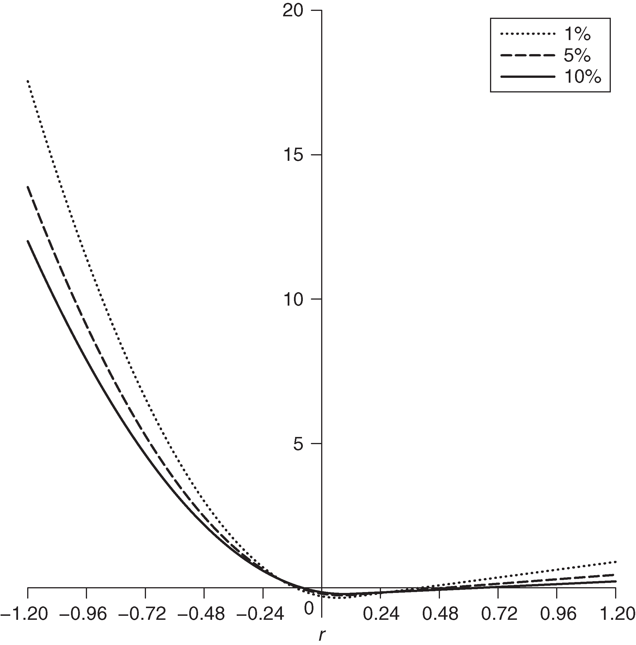
For tail probabilities 0.01, 0.05 and 0.1, the linear term coefficient values are 1.13, 0.65 and 0.40, respectively, and the above influence function is not monotonic decreasing, as is shown in Figure 8 for the case of returns with mean 0.12 and volatility 0.24 (annual mean 12% and volatility 24%). For these three tail probabilities, the use of SSD in place of standard deviation does not completely prevent gains (positive returns) from contributing to risk, but it very considerably reduces this effect.

Figure 8: Nonmonotonic influence function of mean–SSD risk estimator.

Coherence of mean–SSD risk measures

Further exploration of the coefficient of the linear term in (9.8) shows that while it is positive for tail probabilities less than or equal to 0.25, it is negative for tail probabilities as large as or larger than 0.26. Thus, for tail probabilities as large as or larger than 0.26, the influence function ${\mathrm{IF}}_{{\widehat{\mathrm{ES}}}_{\mathrm{SSD}}}(r;F)$ is monotone decreasing, as shown in Figure 7. Lemma 8.1 shows that for such tail probabilities the mean–SSD modified normal distribution parametric ES satisfies the MO coherence axiom and, hence, is coherent (since it always satisfies the PH, SUB and TE axioms).

Figure 9: Monotonic influence functions of mean–SSD risk measure.

Note that for $\gamma =0.01$, $0.05$, $0.10$, $0.26$, $0.50$, $0.56$ the values of $a_{\gamma }=\sqrt{2}\varphi (z_{\gamma }){\gamma }^{-1}$ in (9.4) are $a_{\gamma }=3.77$, $2.92$, $2.48$, $1.76$, $1.13$, $0.996$. Thus, the values of $a_{\gamma }$ fall in the sufficient condition interval  of Fischer’s Lemma 4.1 only for tail probabilities larger than about 0.55. Thus, Fischer’s Lemma 4.1 is not sufficient to obtain our coherence result for $0.26\le \gamma \le 0.55$ and correspondingly $1.0\le a_{\gamma }\le 1.76$, so we have extended the Fischer mean–SSD sufficient condition on $a$ from  to .

Since we only know that mean–SSD is coherent for tail probabilities as large as or larger than 0.26, one might ask: why bother? It seems to us that the results suggest we consider mean–SSD as a nonparametric risk measure for the range  and study its properties in comparison with ES.

Variance of mean–SSD modification of normal distribution ES MLE

Straightforward but tedious calculations provided in Appendix D (available online) show that the asymptotic variance of the mean–SSD estimator is given by

	$V_{{\widehat{\mathrm{ES}}}_{\mathrm{SSD}}}$	$=E[{\mathrm{IF}}_{{\widehat{\mathrm{ES}}}_{\mathrm{SSD}}}^2(r;N)]$
		$=\left[1+\left({\displaystyle \frac{5}{4}}-{\displaystyle \frac{2}{\pi }}\right){\displaystyle \frac{{\varphi }^2(z_{\gamma })}{{\gamma }^2}}\right]{\sigma }^2$
		$\approx \left[1+0.61{\displaystyle \frac{{\varphi }^2(z_{\gamma })}{{\gamma }^2}}\right]{\sigma }^2.$		(9.9)

By way of comparison, the asymptotic variance of a normal distribution ES MLE is

$$V_{{\widehat{\mathrm{ES}}}_{\text{MLE–N}}}=\left[1+0.5\frac{{\varphi }^2(z_{\gamma })}{{\gamma }^2}\right]{\sigma }^2.$$

(9.10)

From the formulas for $V_{{\widehat{\mathrm{ES}}}_{\mathrm{SSD}}}$ and $V_{{\widehat{\mathrm{ES}}}_{\text{MLE–N}}}$, it appears that the standard errors of the two ES estimators are not very different, and this is confirmed in Figure 10. A very small price is paid in terms of estimator standard error for replacing the standard deviation with the SSD in the normal distribution ES MLE.

Figure 10: Mean–SSD versus normal distribution ES MLE asymptotic standard errors.

10 Summary and discussion

We used influence functions as a basic tool in a comparative analysis of nonparametric ES estimators versus parametric ES MLEs, with a focus in the latter case on normal distributions and $t$-distributions. The influence function formulas derived immediately reveal two important differences between nonparametric ES estimators and ES MLEs.

1. (a)

   The former have piecewise linear monotonic decreasing influence functions that have constant small negative values for all sufficiently large returns and are linearly unbounded for all sufficiently negative returns.

2. (b)

   The influence functions of ES MLEs are approximately symmetric and unbounded, which results in the undesirable property that large positive returns indicate large risk.

The formulas also reveal a distinction between the influence functions for normal distribution ES MLE influence functions and $t$-distribution ES MLE influence functions, in that the former are quadratically unbounded and the latter are logarithmically unbounded, thereby reflecting the tail fatness of $t$-distributions relative to normal distributions.

The influence function-based asymptotic variance formulas we derived for ES estimators reveal a very important behavior of asymptotic standard error as a function of ES tail probability: standard errors increase very rapidly as the ES tail probability decreases below 5% (see Figures 4 and 5). In this regard, the Basel III recommendation to use a 2.5% tail probability is prudent (compared with the 1% recommendation for VaR), and one can see that a case could be made for using a 5% tail probability based on the reduction in standard error relative to a 2.5% tail probability.

The asymptotic variance formulas also allow us to assess the asymptotic standard error efficiency of nonparametric ES estimators relative to ES MLEs that achieve the minimum asymptotic variance among consistent estimators. The standard error efficiency in question ranges from approximately 45% to 72% across normal distributions and $t$-distributions with $\text{DOF}=3,5,10$ as well as tail probabilities of 1%, 2.5% and 5%. This is the price that must be paid for the simplicity of nonparametric ES estimators relative to ES MLEs.

The main results of our Monte Carlo study of the finite sample performance of ES estimators are as follows.

1. (1)

   The $t$-distribution ES MLEs are preferred on fundamental statistical grounds and have finite sample standard error formulas that, overall, provide very good finite sample approximations, with some overestimation in the very infrequent event that the returns are normally distributed.

2. (2)

   The standard error estimators for nonparametric ES estimators are only safely usable at a minimum sample size of 400 and a tail probability of 5%, where a small correction is still needed for underestimation.

At the Basel III-recommended 2.5% tail probability, even larger sample sizes are likely needed.

It follows that a risk manager who is confident in the adequacy of $t$-distribution models of returns will be inclined to use a $t$-distribution ES MLE. The question remains whether or not such results can be extended to the family of skewed $t$-distributions that will sometimes, if not frequently, be needed to adequately model returns. As for a risk manager who, in spite of the poor accuracy of their finite sample standard error estimators, wishes to use nonparametric ES estimators, the factor-model Monte Carlo method of Jiang and Martin (2015) provides a way to obtain better standard error estimates for nonparametric ES estimators.

While the ES MLEs and the performance of their standard error estimators are attractive, the lack of monotonicity in their influence functions remains troubling. This led us to study the relationship between ES measure coherence and the monotonicity of an ES estimator influence function, focusing in this paper on the case of normally distributed returns. As a preliminary to this study, we proved (in a lemma) that if there exists a risk measure estimator with an influence function that is monotonic decreasing, then that risk measure satisfies the coherent risk measures monotonicity axiom. We derived the influence function formula for a mean–SSD modification of a normal distribution ES MLE, obtained by replacing the standard deviation with the SSD. We then established a sufficient condition on the multiplier of the SSD such that the influence function is monotonic decreasing and, therefore, the mean–SSD risk measure is coherent.

Since a mean–SSD coherent risk measure is a simple modification of an ES MLE for normal distributions, it is natural to think that one might obtain a useful modification of ES MLEs for $t$-distributions by modifying the scale estimator to be a semi-scale estimator. That this is the case is shown in Martin and Zhang (2017). The risk management applications of those results remain to be studied.

Declaration of interest

The authors report no conflicts of interest. The authors alone are responsible for the content and writing of the paper.

Acknowledgements

Our thanks to a reviewer who both pointed out that in the original version of our paper we ignored the importance of conditional ES and suggested an interesting way to follow the outline of the current paper in writing a paper on conditional ES. We appreciate this suggestion, which we intend to pursue.

R. D. Martin’s research for this paper was supported by the Department of Applied Mathematics at the University of Washington in the form of partial academic year salary for research.

References

• Basel Committee on Banking Supervision (2013). Fundamental review of the trading book. Second Consultative Document, October, Bank for International Settlements. URL: http://www.bis.org/publ/bcbs265.htm.
• Basel Committee on Banking Supervision (2014a). Analysis of the trading book hypothetical portfolio exercise. Report, September, Bank for International Settlements. URL: http://www.bis.org/publ/bcbs288.pdf.
• Basel Committee on Banking Supervision (2014b). Fundamental review of the trading book: outstanding issues. Report, December, Bank for International Settlements. URL: http://www.bis.org/bcbs/publ/d305.htm.
• Bertsimas, D., Lauprete, G. J., and Samarovc, A. (2004). Shortfall as a risk measure: properties, optimization and applications. Journal of Economic Dynamics & Control 28, 1353–1381 (https://doi.org/10.1016/S0165-1889(03)00109-X).
• Cai, Z., and Wang, X. (2008). Nonparametric estimation of conditional VaR and expected shortfall. Journal of Econometrics 147, 120–130 (https://doi.org/10.1016/j.jeconom.2008.09.005).
• Casella, G. and Berger, R. R. (2002). Statistical Inference, 2nd edn. Duxbury Press.
• Chen, X., and Martin, R. D. (2019). Standard errors of risk and performance measures with serially correlated returns. Preprint, Social Science Research Network. URL: https://ssrn.com/abstract=3085672.
• Filippova, A. (1962). Mises theorem on the asymptotic behavior of functionals of empirical distribution functions and its statistical applications. Theory of Probability and Its Applications 7(1), 24–57 (https://doi.org/10.1137/1107003).
• Fischer, T. (2003). Risk capital allocation by coherent risk measures based on one-sided moments. Insurance: Mathematics and Economics 32, 135–146 (https://doi.org/10.1016/S0167-6687(02)00209-3).
• Hampel, F. R. (1974). The influence curve and its role in robust estimation. Journal of American Statistical Association 69, 383–393 (https://doi.org/10.1080/01621459.1974.10482962).
• Hampel, F. R., Ronchetti, E. M., Rousseeuw, P. J., and Stahel, W. A. (1986). Robust Statistics: The Approach Based on Influence Functions. Wiley.
• Heidelberger, P., and Welch, P. D. (1981). A spectral method for confidence interval generation and run length control in simulations. Communications of the ACM 24(4), 233–245 (https://doi.org/10.1145/358598.358630).
• Huber, P. J., and Ronchetti, E. M. (2009). Robust Statistics, 2nd edn. Wiley (https://doi.org/10.1002/9780470434697).
• Jiang, Y., and Martin, R. D. (2015). Better risk and performance estimates with factor-model Monte Carlo. The Journal of Risk 17(5), 1–39 (https://doi.org/10.21314/JOR.2015.311).
• Jorion, P. (2007). Value-at-Risk, 3rd edn. McGraw-Hill.
• Krokhmal, P. A. (2007). Higher moment coherent risk measures. Quantitative Finance 7(4), 373–387 (https://doi.org/10.1080/14697680701458307).
• Lange, K. L., Little, R. J. A., and Taylor, J. M. G. (1989). Robust statistical modeling using the $t$-distribution. Journal of the American Statistical Association 84, 881–896 (https://doi.org/10.2307/2290063).
• Lucas, A. (1997). Robustness of the student $t$ based $M$-estimator. Communications in Statistsics: Theory and Methods 26(5), 1165–1182 (https://doi.org/10.1080/03610929708831974).
• Maronna, R., Martin, R. D., and Yohai, V. J. (2006). Robust Statistics: Theory and Methods. Wiley (https://doi.org/10.1002/0470010940).
• Martin, R. D., and Zhang, S. (2017). A $t$-distribution $M$-estimator of expected shortfall based on a semi-scale estimator. Working Paper.
• Martins-Filho, C., and Yao, F. (2006). Estimation of value-at-risk and expected shortfall based on nonlinear models of return dynamics and extreme value theory. Studies in Nonlinear Dynamics & Econometrics 10(2), 1–41 (https://doi.org/10.2202/1558-3708.1304).
• Martins-Filho, C., Yao, F., and Torero, M. (2018). Nonparametric estimation of conditional value-at-risk and expected shortfall based on extreme value theory. Econometric Theory 34, 23–67 (https://doi.org/10.1017/S0266466616000517).
• McNeil, A. J., and Frey, B. (2000). Estimation of tail-related risk measures for heteroscedastic financial time series: an extreme value approach. Journal of Empirical Finance 7, 271–300 (https://doi.org/10.1016/S0927-5398(00)00012-8).
• McNeil, A. J., Frey, R., and Embrechts, P. (2015). Quantitative Risk Management, revised edn. Princeton University Press.
• Newey, W. K., and West, K. D. (1987). A simple, positive semi-definite, heteroskedasticity and autocorrelation consistent covariance matrix. Econometrica 55(3), 703–708 (https://doi.org/10.2307/1913610).
• Newey, W. K., and West, K. D. (1994). Automatic lag selection in covariance matrix estimation. Review of Economic Studies 61(4), 631–653 (https://doi.org/10.2307/2297912).
• Rockafellar, R. T., and Uryasev, S. (2000). Optimization of conditional value-at-risk. The Journal of Risk 2(3), 21–41 (https://doi.org/10.21314/JOR.2000.038).
• Scandolo, G. (2015). An introduction to coherent risk measures. Presentation, Risk Measures: Frontiers of Mathematics and Regulations, Università di Bologna.
• Zhang, S. (2016). Three equivalent expressions for $t$-distribution expected shortfall. Preprint, Social Science Research Network. URL: https://ssrn.com/abstract=2883935.
• Zhang, S., and Green, C. G. (2017). The univariate $t$-distribution information matrix. Preprint, Social Science Research Network (https://doi.org/10.2139/ssrn.3086998).

Download PDF Appendix 1

• Keywords
• Asymptotic theory
• Expected shortfall
• Maximum likelihood estimation
• Parametric modelling
• Original research
• More
  Less