What do central counterparty default funds really cover? A network-based stress test answer

Giulia Poce, Giulio Cimini, Andrea Gabrielli, Andrea Zaccaria, Giuditta Baldacci, Marco Polito, Mariangela Rizzo and Silvia Sabatini

Abstract

In recent years, an increased effort has been made to further the development of effective stress tests that can be used to quantify the resilience of financial institutions. Here, we propose a stress test methodology for central counterparties (CCPs) based on a network characterization of clearing members (CMs) that takes into account the propagation and amplification of financial distress through the network of bilateral exposures between CMs. We apply the proposed framework to the fixed-income asset class of Cassa di Compensazione e Garanzia (CC&G), the CCP operating in Italy, whose cleared securities are mainly Italian government bonds. We consider two different scenarios where exogenous losses may be incurred: a distributed initial shock and a shock corresponding with the cover 2 regulatory requirement (entailing the simultaneous default of the two most exposed CMs). Network effects turn out to substantially increase the vulnerability of the CMs in both scenarios, though distress propagation is much more rapid in the latter case, where we note a large number of early triggered additional defaults. This shows that setting a default fund to cover insolvencies on a cover 2 basis alone may not be adequate for the taming of systemic events. Overall, our network-based stress test methodology represents a refined tool for calibrating conservative default fund amounts.
 

Download PDF Appendix 1

Introduction

1 Introduction

The financial crises of the last decade exposed the structural fragility of the financial system, providing the impetus for the considerable scientific effort that has been made to characterize the complex patterns of interconnections resulting from direct and indirect exposures between financial institutions (see, for example, Boss et al 2004; Nier et al 2007; Iori et al 2008). Many studies have focused on understanding how local events may trigger global instability through the spreading and amplification of financial distress, with the aim of quantifying the resulting systemic risk in capital markets. The relevant literature ranges from the seminal works of Allen and Gale (2000), Eisenberg and Noe (2001) and Furfine (2003) to the recent contributions of Acemoglu et al (2015) and Battiston et al (2016a, 2016b). At the same time, regulators were pushed to introduce more stringent microprudential rules around capital and liquidity requirements that, together with the implementation of extraordinary monetary policies, eventually increased the robustness of the financial system.

Central counterparties (CCPs) contribute to the stability of the system (Duffie and Zhu 2011) by acting as contract intermediaries between financial institutions, which take the name of clearing members (CMs). To fulfil this function, a CCP collects guarantees from its CMs in the form of daily margins that are used to cover any potential liquidation costs incurred by the insolvency of a CM as well as in the form of default fund amounts that may be used to manage market risk above the level covered by the margins (Cumming and Noss 2013; Nahai-Williamson et al 2013; Murphy and Nahai-Williamson 2014). According to European Market Infrastructure Regulation (EMIR), the default fund should be calibrated via various stress tests ensuring compliance with the cover 2 requirement; that is, the CCP must be able to withstand any losses resulting from the default of the two CMs to which it is most exposed. (For further details, see EMIR Regulation (EU) 648/2012 on over-the-counter (OTC) derivatives, CCPs and trade repositories, available at https://bit.ly/2yyiSgO.)

The European Securities and Markets Authority (ESMA) recently coordinated the first assessment across the European Union (EU) of CCP resilience to “extreme but plausible” market developments (for the full report on ESMA’s EU-wide CCP stress test, published in April 2016, we refer the reader to https://bit.ly/2Ec7KMA). This stress exercise focused on the counterparty risk that CCPs would face as a result of multiple CM defaults and simultaneous market price shocks. The assessment also included spillover losses associated with the default waterfall mechanism (Article 45, EMIR); that is, if the guarantees posted by the defaulted CMs are insufficient to cover the total liquidation costs, guarantees posted by nondefaulting CMs will be used too. Spillover losses may also arise because the various CCPs are highly interconnected through common CMs. Although the ESMA exercise found the EU’s system of CCPs to be resilient overall, it also highlighted that an important protection for CCPs is provided by the resources posted by nondefaulting CMs, which are thus themselves at risk of facing significant losses. In severe scenarios, this could trigger second-round effects via additional losses and defaults. This is why ESMA recommended that CCPs carefully evaluate the creditworthiness of their CMs as well as their potential exposures due to their participation with other CCPs.

We address this call by developing a network-based stress test framework. Tailored to the needs of CCPs, it takes into account contagion effects among CMs due to the reverberation of credit and liquidity shocks over the network of bilateral exposures that exists between them. In doing so, we aim to overcome the current definition of the CCP stress tests used to determine the size of their default funds. In particular, we quantitatively challenge the cover 2 rule by assessing the systemic losses that the default of two CMs may generate as side effects, and by considering whether these losses are comparable to those arising from a distributed macroeconomic shock. Instead of fixing ex ante the number of CMs that might default at the same time, we follow an ex post approach, determining how many CMs would be affected by a given initial shock. Due to the difficulties of collecting (at CCP level) the data needed to assess the exposures of the CCP’s CMs to other CCPs, we focus on a single cleared market, namely, the fixed-income asset class of Cassa di Compensazione e Garanzia (CC&G), the only Italian EMIR-authorized clearing house.¹¹The cleared products we consider include Italian government bonds, repurchase agreements (repos) and corporate bonds traded on Borsa Italiana platforms. The fixed-income asset class is the most significant in terms of cleared volumes and systemic importance in the Italian financial system.${}^{,}$²²For a complete description of CC&G’s current stress test methodology, please refer to https://bit.ly/2A4PC37. Note that CC&G’s current fixed-income default fund is generally gauged on a cover 4 basis (covering the four members with the largest recorded exposures) via a more conservative process than that prescribed by the cover 2 requirement.³³CC&G’s default waterfall, including both the margins and the default fund, has been designed in compliance with both EMIR and the Committee on Payment and Settlement Systems–Technical Committee of the International Organization of Securities Commissions (CPSS–IOSCO) Principles for Financial Market Infrastructures (2012).

2 A network-based stress test

To summarize, our stress test methodology is based on the assessment of the financial positions and the interconnections between CMs participating in the market cleared by CC&G. This information is then used to compute the equity losses sustained by the CMs due to an initial idiosyncratic and macroeconomic shock reverberating through the bilateral exposures of the CMs in the form of credit and liquidity shocks. The proposed stress test framework is thus made up of four fundamental steps that are briefly outlined below. Full details of the method can be found in Poce et al (2016).

(1) Assessment of daily balance sheets through a Merton-like model

The financial position of a given CM $i$ (belonging to CC&G’s fixed-income asset class) at date $t$ is summarized by the balance sheet identity

$$E_i(t)=A_i(t)-L_i(t),$$

(2.1)

where $A_i(t)$ and $L_i(t)$ represent total assets and liabilities, respectively. CM $i$ is considered solvent as long as its equity $E_i(t)$ is positive. Starting from the information disclosed periodically in their balance sheets, we compute the financial positions of the CMs using a Merton-like model (Merton 1974). Crucially, we suppose that a default occurs the first time a firm’s total assets fall below the default point; thus, following Tudela and Young (2005), we estimate the equity as the price of a down-and-out call option on the assets of the firm, with a strike price equal to the notional amount of issued debt. The option value $E_i(t)$ is retrieved from the market as the firm’s market capitalization, from which we can determine the current value of assets $A_i(t)$ and liabilities $L_i(t)$ (see the online appendix).

(2) Building a network of inter-clearing member exposures

In order to build the network of bilateral exposures between CMs, we first determine the daily values of the inter-CM assets $A_i^{\mathrm{INT}}(t)$ and liabilities $L_i^{\mathrm{INT}}(t)$ (resulting from direct credits and debits among CMs). To do so, we use the interbank assets and liabilities reported on the balance sheet as proxies for these two quantities. Further, we assume that, for each CM, the proportion of interbank assets (liabilities) over total assets (liabilities) remains constant over time (Nier et al 2007). Individual contract values are then inferred through the fitness-induced maximum entropy approach of Cimini et al (2015); the amount $a_{ij}^{\mathrm{INT}}(t)$ of the loan granted by $i$ to $j$ at $t$ can be expressed as⁴⁴See Anand et al (2018) for a recent comparative overview of network reconstruction methods.

	$a_{ij}^{\mathrm{INT}}(t)$	$={\displaystyle \frac{z^{-1}+A_i^{\mathrm{INT}}(t)L_j^{\mathrm{INT}}(t)}{C^{\mathrm{INT}}(t)}}{\omega }_{ij}(t),$
	${\omega }_{ij}(t)$			(2.2)

where ${\omega }_{ij}(t)$ denotes the presence of the link, $C^{\mathrm{INT}}(t)={\sum }_i{A}_i^{\mathrm{INT}}(t)$ is the total volume of the inter-CM market and $z$ is a parameter that controls for the density of the network.⁵⁵Here, we set $z$ to have a network density of 5%, like that observed in the Italian interbank market e-MID on a daily aggregation scale (Finger et al 2013).${}^{,}$⁶⁶In principle, CMs may establish contracts with other CMs as well as external firms; the latter might be included in the network in the form of links pointing out of the system. We use Bank for International Settlements (BIS) locational banking statistics (https://bit.ly/2Eoq99c) to estimate that the foreign positions of Italian banks are rather small (amounting to roughly 10% of the total exposure) and can therefore be neglected in our analysis.

(3) Simulation of initial shocks

We model two different types of initial shock hitting the market.

Distributed shock

To model a distributed distress, we decrease the equity of each CM by

$$S_i(t)=\{[\varphi {\xi }_i(t)+(1-\varphi )]xC(t)+\max [M_i^{\mathrm{STR}}(t)-M_i(t),0]\}\frac{E_i(t)}{{\sum }_j{E}_j(t)}.$$

(2.3)

The first term is an exogenous shock on external assets, which we model using an idiosyncratic component and a macroeconomic component (Manna and Schiavone 2012), both affecting the CM in a way that is proportional to its equity.⁷⁷The stochastic term is given by the Poisson variable ${\xi }_i(t)\sim ?(1)$. Without loss of generality, we use $\varphi =\frac{1}{2}$. The magnitude of the shock is set by the parameter $x$, namely, the average total exogenous shock over the total market volume $C(t)={\sum }_i{A}_i(t)$. The second term represents the hypothetical liquidity pressure resulting from the higher margins required by CC&G in stressed conditions; this term is quantified as the difference between $M_i^{\mathrm{STR}}(t)$ (ie, the margins posted under conservative stress scenarios) and $M_i(t)$ (ie, the margins actually posted by the CM).⁸⁸This term is also rescaled to obtain margin increases comparable to CM equities. Overall, we consider only shocks that actually cause decreases in equity, imposing $S_i(t)=0$ whenever .

Cover 2 shock

To fit with the cover 2 EMIR requirement, we simulate a scenario where the initial shock is the straight simultaneous default of CMs $\tilde{i}$ and $\tilde{j}$ (that is, the two CMs to which CC&G has the largest exposure). Thus, we obtain

$$S_{\tilde{i}}(t)=E_{\tilde{i}}(t),S_{\tilde{j}}(t)=E_{\tilde{j}}(t),S_k(t)=0\mathit{\hspace{1em}}\text{for all }k\ne \tilde{i},\tilde{j}.$$

(2.4)

(4) Reverberation of credit and liquidity shocks

Initial shocks reverberate throughout the network of bilateral exposures between CMs, causing additional losses according to two main mechanisms (Chan-Lau et al 2009). They are

• •

  credit shocks, where CMs can fail to meet obligations, resulting in actual losses for creditors; and

• •

  liquidity shocks, where CMs can start to hoard liquidity, driving other CMs to restore their liquidity provisions by fire selling their illiquid assets at a discount.⁹⁹The burst of the interest rate spread between long-term and overnight loans represents another liquidity hoarding spillover that can hinder the refinancing of assets through long-term loans.

These shocks propagate even if no default has occurred, as experiencing equity losses brings a CM “closer” to default, implying a decrease in both the value of its obligations (Bardoscia et al 2015) and its capability (or willingness) to lend money to the market (Cimini and Serri 2016). To quantify the resulting losses that propagate to other CMs, we define the impact of $j$ on $i$ as

$$W_{i\leftarrow j}(t)=\frac{\lambda a_{ij}^{\mathrm{INT}}(t)+\rho \gamma (t)a_{ji}^{\mathrm{INT}}(t)}{E_i(t)},$$

(2.5)

where $0\le \lambda \le 1$ is the loss given default, $0\le \rho \le 1$ is the fraction of the lost liquidity that is to be replenished by asset sales and $\gamma (t)$ quantifies asset depreciation during the fire sales. According to Bardoscia et al (2015) and Cimini and Serri (2016), the dynamics of shock propagation consist of several rounds $\{n\}$. In each of these rounds, we iteratively spread individual distress levels given by the relative changes in equity $h_i^{[n]}(t)=1-E_i^{[n]}(t)/E_i^{[0]}(t)$ and weighted by the wealth potentially affected.

• •

  At step $n=0$, the system is experiencing no distress. Hence, $E_i^{[0]}(t)\equiv E_i(t)\Rightarrow h_i^{[0]}(t)=0$ for all $i$.

• •

  At step $n=1$, the initial shock hits the market so that $E_i^{[1]}(t)\equiv E_i(t)-S_i(t)\Rightarrow h_i^{[1]}(t)=S_i(t)/E_i(t)$ for all $i$.

• •

  At steps $n>1$, $h$ values are obtained by iterating the equation for the evolution of the CM’s equity as follows:

  	$h_i^{[n+2]}(t)$	$=\min \{1,h_i^{[n+1]}(t)+{\displaystyle \sum _{j\in ?[n+1]}}{\displaystyle \frac{\lambda a_{ij}^{\mathrm{INT}}(t)+\rho {\gamma }^{[n]}(t)a_{ji}^{\mathrm{INT}}(t)}{E_i^{[0]}(t)}}$
  		$\mathrm{\hspace{1em}\hspace{1em}}\mathit{\hspace{1em}\hspace{1em}\hspace{1em}\hspace{1em}\hspace{1em}\hspace{1em}\hspace{1em}\hspace{1em}\hspace{1em}\hspace{1em}\hspace{1em}\hspace{1em}}\times [h_j^{[n+1]}(t)-h_j^{[n]}(t)]\},$		(2.6)

where we assume that equity losses for CM $j$ translate linearly into equity losses for CM $i$.¹⁰¹⁰Linearity is the simplest possible assumption when the real functional form is unknown. However, our methodology can easily be extended to generic convex functions of the equity loss, as in Bardoscia et al (2016). What we observe in these cases (at least when the function is not so close to zero for small losses, so that shocks can actually propagate) is a difference in the model dynamics in the early stages. This difference, however, vanishes as stationarity approaches, corresponding to the extreme scenario with no policy intervention. As a CCP needs to be able to gauge the default fund on a very conservative basis, linearity seems a more appropriate hypothesis.

In the above expression, denotes the set of CMs that have not defaulted up to iteration $n$. These CMs may still spread their financial distress (note that $h_i=1$ signals the default of $i$). The aggregate amount of inter-CM assets that may potentially be liquidated at $n$ is given by

$$Q^{[n]}(t)=\sum _{j\in ?[n+1]}\sum _k{a}_{jk}^{\mathrm{INT}}(t)[h_j^{[n+1]}(t)-h_j^{[n]}(t)]$$

so that the fire sale devaluation factor is ${\gamma }^{[n]}(t)={\{C^{\mathrm{INT}}(t)/[\rho Q^{[n]}(t)]-1\}}^{-1}$. The dynamics stop at $n^{*}$ when no more CMs can propagate their distress. The set of vulnerabilities ${\{h_i^{[*]}(t)\}}_{i\in N}$ then quantifies the final potential equity losses of CMs.

3 Results

We now illustrate the results of the application of our proposed network-based stress test methodology to the fixed-income market cleared by CC&G.¹¹¹¹Input data for the stress test exercise is taken from the CMs’ most recent balance sheet information (available as of September 2016) as well as CC&G’s fixed-income margins (collected between July and October 2016). The results presented in this paper refer to a specific date in such a range. Our particular choice of date, however, does not significantly alter our results because, throughout the relevant period, we observe small changes in the total uncovered exposures of the two most exposed CMs (10%) and in the default fund (11%). These variations are in line with those obtained over a longer time period (between September 2015 and October 2016), for which the change in the total uncovered exposures of the two most exposed CMs is 15%, while that of the default fund is 10%.${}^{,}$¹²¹²The results obtained are averages over an ensemble of 1000 realizations of steps (2)–(4) of our framework. Thanks to the numerosity of the ensemble, relative confidence intervals become negligible and are not displayed in the plots. We omit the explicit dependence of quantities on the chosen date $t$.

3.1 Dynamics of clearing member vulnerabilities

In order to show how the method works in detail, we start with a specific case study and set $\lambda =0.6$ (the average loss given default value observed for CC&G’s CMs) and $\rho =0.6$ (set homogeneously with $\lambda$). We compare three quantities for each CM $i$, namely:

• •

  $h_i^{[1]}$, the vulnerability, or relative equity loss, given by the initial shock;

• •

  $h_i^{[2]}$, the vulnerability after the first network reverberation of shocks (ie, the second-round relative loss); and¹³¹³Note that stopping the dynamics in the early rounds in this way models corrective actions that might reasonably be expected to be implemented by regulators.

• •

  $h_i^{[*]}$, the vulnerability after the network propagation of shocks has been exhausted.

Figure 1: Individual vulnerability $h_i$ versus leverage value ${\mathrm{\Lambda }}_i=A_i^{\mathrm{INT}}/E_i$ for each CM $i$. The histograms report, for all $i$, the triplet $h_i^{[\text{1}]}$ (initial relative equity loss), $h_i^{[\text{2}]}$ (second-round loss caused by the first network reverberation) and $h_i^{[*]}$ (the final loss when the network reverberation of shocks has been exhausted). (a) The scenario of distributed initial shocks from (2.3) with $x={\text{10}}^{-\text{3}}$. (b) The scenario of cover 2 initial shocks from (2.4). In both cases, we set $\lambda =\rho =\text{0.6}$.

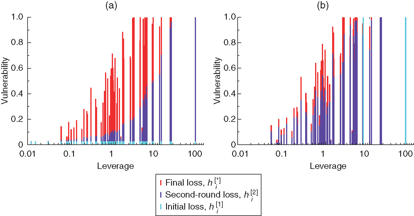
By construction, $h_i^{[1]}\le h_i^{[2]}\le h_i^{[*]}$. Figure 1 shows these values for two scenarios, entailing initial shocks that are (a) distributed (with $x={10}^{-3}$) and (b) cover 2.¹⁴¹⁴The rationale behind this choice of $x$ is detailed in the next subsection. The first observation that strikes us is the significance of network effects, which are diverse among CMs and generally amplify losses significantly. The considerable variation in initial shock conditions gives rise to very different configurations in the early stages of the shock propagation dynamics ($n=2$); if, however, shocks continue to propagate ($n=n^{*}$), then the system falls into similar stationary configurations. This is consistent with initial shocks leading to similar initial equity losses ($2.6\%$ and $3.0\%$, on average, for the distributed and cover 2 cases, respectively). In the scenario entailing distributed initial shocks, the system remains mostly stable after the first network reverberation round, and CMs with greater inter-CM leverage values ${\mathrm{\Lambda }}_i=A_i^{\mathrm{INT}}/E_i$ are generally characterized by greater vulnerabilities. However, as shocks continue to propagate, several CMs come very close to default, with a dependency of vulnerability on leverage that is still evident.¹⁵¹⁵Note that a CM can default due to shock reverberation only if its inter-CM leverage is greater than 1. Indeed, we see that the value $\mathrm{\Lambda }=1$ qualitatively separates a regime of low losses from a regime of high losses. If we consider the defaulted CMs in this extreme scenario, their total uncovered exposure (ie, the guarantees that they require, in addition to those already posted, to cover a hypothetical stressed margin call, as calculated in CC&G’s stress test) is €3.0 billion. We obtain comparable results for the cover 2 scenario, in which the total uncovered exposure of defaulted CMs is €3.2 billion. Both are well covered by CC&G’s default fund at the date (€3.5 billion), which, however, is gauged far more conservatively than prescribed by the cover 2 rule. Indeed, the fact that the default of the two CMs is equivalent in terms of loss to a plausible distributed shock, and can lead to additional defaults, shows that gauging the default fund solely on a cover 2 basis may not be conservative enough.

3.2 Stability analysis

We generalize our results by studying the stability regime of the market with the use of the residual default fund ratio $R_{\mathrm{DF}}^{[n]}$; this tells us the fraction of the default fund that remains after we have subtracted the uncovered exposures of the defaulted CMs (ie, those with $h^{[n]}=1$).¹⁶¹⁶Here, we adopt a conservative approach that does not consider the netting of liabilities in case of default. This means that if two or more CMs default at the same time, we assume that the CCP needs to liquidate all of its positions, without taking into account any possible netting benefit between the different CMs. We recall that CC&G’s default fund is gauged on a cover 4 basis and is thus much larger than prescribed by regulation based on the cover 2 requirement.

Figure 2: Color map of the residual default fund ratio $R_{\text{DF}}^{[n]}$ depending on the magnitude of the distributed initial shocks $x$ and the shock reverberation through network $n$. $\lambda$ and $\rho$ are both set to 0.6. This kind of analysis can be performed only for the distributed shocks scenario; however, as Figure 1 has already shown, for large values of $n$, systemic losses are also representative of the cover 2 scenario with a similar overall magnitude of initial shocks. Note that the shock propagation dynamics usually converge after a few iterations $n$.

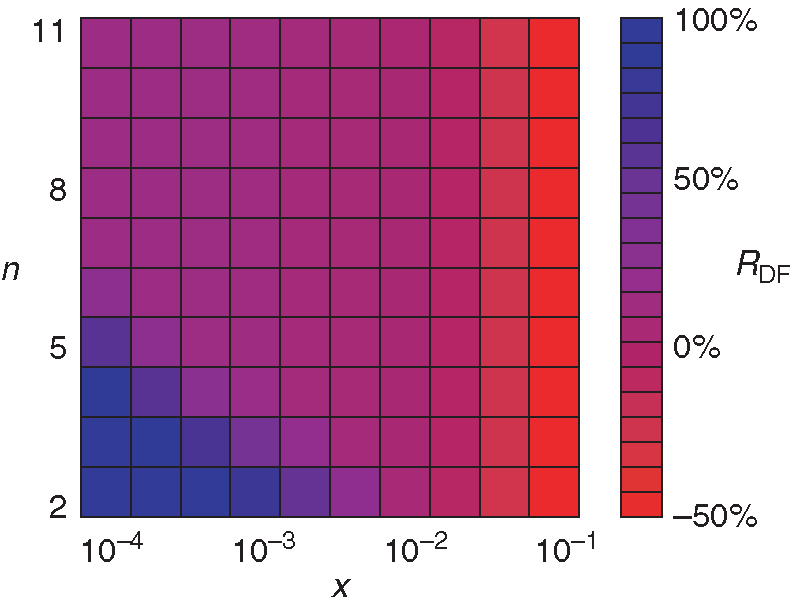
First, we study how the residual default fund varies as a function of the magnitude $x$ of the distributed initial shock and of the progressive network reverberations $n$ (Figure 2). We find that CC&G’s default fund succeeds in covering all exposures in almost every scenario, except where unreasonably high values of $x$ are recorded. To catch the range of plausible values for $x$, we can assume that losses arising from nonperforming loans (NPLs) recorded in the market are likely the result of losses in the value of assets following an initial shock. In particular, the yearly increase (for 2014–15) in losses from NPLs sustained by Italian banks ranges from 1.37% (incorporating the cases where such losses were reduced) to 2.5% (considering only the increase in losses). Using these values as initial vulnerabilities and inverting (2.3), we obtain .

Figure 3: Color map of the (final) residual default fund ratio $R_{\text{DF}}^{[n^{*}]}$ depending on the magnitude of credit and liquidity shocks, given by the loss given default $\lambda$ and the lost funding replenishment ratio $\rho$, respectively. (a) The scenario of distributed initial shocks with $x={\text{10}}^{-\text{3}}$. (b) The scenario of cover 2 initial shocks.

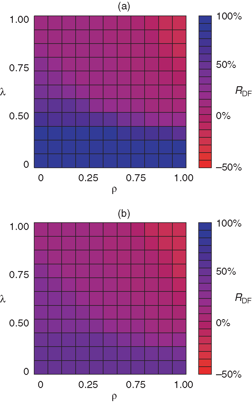
We then assess the system stability with respect to the intensity of credit and liquidity shocks set by the parameters $\lambda$ and $\rho$. The case $n=n^{*}$ turns out to be the most interesting. Figure 3 shows a rather smooth transition between the regimes of low and high losses, with the CC&G default fund becoming insufficient for only very high values of $\lambda$ and $\rho$ (the worst-case total uncovered exposure would be around 18% of the original default fund). This region corresponds, however, to very intense and rather unrealistic shocks, which would mean CMs losing the full amount of any loan made to their defaulted counterpart and having no means of recovering liquidity other than fire selling their assets. Note that in the cover 2 scenario, the default fund is at least halved by covering the two most exposed CMs. Overall, CC&G’s default fund is appropriate in a wide range of economic scenarios because it is more conservatively gauged than that prescribed by the cover 2 requirement.

4 Summary

We proposed a network-based stress test methodology for CCPs aimed at assessing the proportion of equity at risk from their CMs. The model is based on a network characterization of direct credits and debits among CMs as well as the propagation of financial distress mediated by these connections, that is, equity losses caused by an initial shock with both exogenous and endogenous components reverberating within the network (in the form of credit and liquidity shocks) and becoming amplified. We applied the proposed framework to a real case study, namely, the fixed-income asset class of CC&G, the CCP operating in Italy, whose cleared securities are mainly Italian government bonds. We considered two different scenarios: a distributed initial shock as well as a shock corresponding to the cover 2 regulatory requirement (namely, the simultaneous default of the two most exposed CMs). In a nutshell, we found that network effects lead to significant losses and even additional defaults, neither of which should be neglected when calibrating default fund amounts. According to our results, setting the default fund to cover insolvencies on a cover 2 basis alone is not always adequate for taming systemic events; that is, only very conservative default funds can withstand total losses due to the propagation of shocks. In this respect, the fixed-income default fund of CC&G, gauged on a cover 4 basis, appears to be conservative enough. Overall, our network-based stress test can be deemed a refined tool for calibrating default fund amounts.

This model represents an advancement compared with existing stress testing methodologies as well as a response to ESMA’s call for an innovative modeling of interconnections in the financial system. The model can also be extended to cover multiple asset classes within the same CCP or to CMs belonging to multiple CCPs (Cont 2015; Vicente et al 2015; Glasserman et al 2016; Barker et al 2017). This would allow us to build a fully comprehensive stress testing framework that considers the whole financial landscape as a single system made up of interconnected clearing houses and members.

Declaration of interest

The authors report no conflicts of interest. The authors alone are responsible for the content and writing of the paper. The information and views set out in this paper are those of the authors and do not reflect the opinion of CC&G S.p.A., London Stock Exchange Group.

Acknowledgements

This work was supported by the EU projects GrowthCom (FP7-ICT, Grant 611272) and DOLFINS (H2020-EU.1.2.2, Grant 640772) as well as the Italian PNR project CRISIS-Lab. The funders had no role in the design of our study, data collection/analysis, the decision to publish or the preparation of the manuscript. This work was made possible thanks to the support provided by Paolo Cittadini and his colleagues at CC&G.

References

• Acemoglu, D., Ozdaglar, A., and Tahbaz-Salehi, A. (2015). Systemic risk and stability in financial networks. American Economic Review 105(2), 564–608 (https://doi.org/10.1257/aer.20130456).
• Allen, F., and Gale, D. (2000). Financial contagion. Journal of Political Economy 108(1), 1–33 (https://doi.org/10.1086/262109).
• Anand, K., van Lelyveld, I., Banai, A., Christiano Silva, T., Friedrich, S., Garratt, R., Halaj, G., Hansen, I., Howell, B., Lee, H., Martínez Jaramillo, S., Molina-Borboa, J., Nobili, S., Rajan, S., Rubens Stancato de Souza, S., Salakhova, D., and Silvestri, L. (2018). The missing links: a global study on uncovering financial network structure from partial data. Journal of Financial Stability 35, 107–119 (https://doi.org/10.1016/j.jfs.2017.05.012).
• Bardoscia, M., Battiston, S., Caccioli, F., and Caldarelli, G. (2015). Debtrank: a microscopic foundation for shock propagation. PLoS ONE 10(6), e0130406 (https://doi.org/10.1371/journal.pone.0130406).
• Bardoscia, M., Caccioli, F., Perotti, J. I., Vivaldo, G., and Caldarelli, G. (2016). Distress propagation in complex networks: the case of non-linear debtrank. PLoS ONE 11(10), e0163825 (https://doi.org/10.1371/journal.pone.0163825).
• Barker, R., Dickinson, A., Lipton, A., and Virmani, R. (2017). Systemic risk in CCP networks. Risk.net, January 5. URL: http://bit.ly/2CDYgs8.
• Battiston, S., Caldarelli, G., May, R., Roukny, T., and Stiglitz, J. E. (2016a). The price of complexity in financial networks. Proceedings of the National Academy of Sciences of the United States of America 113(36), 10031–10036 (https://doi.org/10.1073/pnas.1521573113).
• Battiston, S., Farmer, J. D., Flache, A., Garlaschelli, D., Haldane, A. G., Heesterbeek, H., Hommes, C., Jaeger, C., May, R., and Scheffer, M. (2016b). Complexity theory and financial regulation. Science 351(6275), 818–819 (https://doi.org/10.1126/science.aad0299).
• Bharath, S. T., and Shumway, T. (2008). Forecasting default with the Merton distance to default model. Review of Financial Studies 21(3), 1339–1369 (https://doi.org/10.1093/rfs/hhn044).
• Boss, M., Elsinger, H., Summer, M., and Thurner, S. (2004). Network topology of the interbank market. Quantitative Finance 4(6), 677–684 (https://doi.org/10.1080/14697680400020325).
• Chan-Lau, J. A., Espinosa, M., Giesecke, K., and Solé, J. A. (2009). Assessing the systemic implications of financial linkages. In IMF Global Financial Stability Report, Volume 2. IMF Monetary and Capital Markets Development. International Monetary Fund. URL: http://ssrn.com/abstract=1417920.
• Cimini, G., and Serri, M. (2016). Entangling credit and funding shocks in interbank markets. PLoS ONE 11(8), e0161642 (https://doi.org/10.1371/journal.pone.0161642).
• Cimini, G., Squartini, T., Garlaschelli, D., and Gabrielli, A. (2015). Systemic risk analysis on reconstructed economic and financial networks. Scientific Reports 5, 15758 (https://doi.org/10.1038/srep15758).
• Cont, R. (2015). The end of the waterfall: default resources of central counterparties. Journal of Risk Management in Financial Institutions 8(4), 365–389. URL: https://bit.ly/2yIW1zd.
• Cumming, F., and Noss, J. (2013). Assessing the adequacy of CCPs’ default resources. Financial Stability Paper 26, Bank of England. URL: https://bit.ly/2CFfNQP.
• Duffie, D., and Zhu, H. (2011). Does a central clearing counterparty reduce counterparty risk? Review of Asset Pricing Studies 1(1), 74–95 (https://doi.org/10.1093/rapstu/rar001).
• Eisenberg, L., and Noe, T. H. (2001). Systemic risk in financial systems. Management Science 47(2), 236–249 (https://doi.org/10.1287/mnsc.47.2.236.9835).
• Finger, K., Fricke, D., and Lux, T. (2013). Network analysis of the e-MID overnight money market: the informational value of different aggregation levels for intrinsic dynamic processes. Computational Management Science 10(2–3), 187–211 (https://doi.org/10.1007/s10287-013-0171-9).
• Furfine, C. H. (2003). Interbank exposures: quantifying the risk of contagion. Journal of Money, Credit and Banking 35(1), 111–128 (https://doi.org/10.1353/mcb.2003.0004).
• Glasserman, P., Moallemi, C. C., and Yuan, K. (2016). Hidden illiquidity with multiple central counterparties. Operations Research 64(5), 1143–1158 (https://doi.org/10.1287/opre.2015.1420).
• Iori, G., Masi, G. D., Precup, O. V., Gabbi, G., and Caldarelli, G. (2008). A network analysis of the italian overnight money market. Journal of Economic Dynamics & Control 32(1), 259–278 (https://doi.org/10.1016/j.jedc.2007.01.032).
• Jones, E. P., Mason, S. P., and Rosenfeld, E. (1984). Contingent claims analysis of corporate capital structures: an empirical investigation. Journal of Finance 39(3), 611–625 (https://doi.org/10.2307/2327920).
• Manna, M., and Schiavone, A. (2012). Externalities in interbank network: results from a dynamic simulation model. Temi di Discussione 893, Bank of Italy. URL: https://bit.ly/2Ck9fG0.
• Merton, R. C. (1974). On the pricing of corporate debt: the risk structure of interest rates. Journal of Finance 29(2), 449–470 (https://doi.org/10.2307/2978814).
• Murphy, D., and Nahai-Williamson, P. (2014). Dear Prudence, won’t you come out to play? Approaches to the analysis of central counterparty default fund adequacy. Financial Stability Paper 30, Bank of England. URL: https://bit.ly/2EshkLx.
• Nahai-Williamson, P., Ota, T., Vital, M., and Wetherilt, A. (2013). Central counterparties and their financial resources: a numerical approach. Financial Stability Paper 19, Bank of England. URL: https://bit.ly/2IZoFzJ.
• Nier, E. W., Yang, J., Yorulmazer, T., and Alentorn, A. (2007). Network models and financial stability. Journal of Economic Dynamics and Control 31(6), 2033–2060 (https://doi.org/10.1016/j.jedc.2007.01.014).
• Poce, G., Cimini, G., Gabrielli, A., Zaccaria, A., Baldacci, G., Polito, M., Rizzo, M., and Sabatini, S. (2016). What do central counterparties default funds really cover? A network-based stress test answer. Preprint (arXiv:1611.03782v1).
• Tudela, M., and Young, G. (2005). A Merton-model approach to assessing the default risk of UK public companies. International Journal of Theoretical and Applied Finance 8(6), 737–761 (https://doi.org/10.1142/s0219024905003256).
• Vicente, L., Cerezetti, F., Faria, S. D., Iwashita, T., and Pereira, O. (2015). Managing risk in multi-asset class, multimarket central counterparties: the core approach. Journal of Banking & Finance 51, 119–130 (https://doi.org/10.1016/j.jbankfin.2014.08.016).

Download PDF Appendix 1

• Keywords
• CCP
• Default funds
• Network theory
• Stress-testing
• Systemic risk
• Original research