Journal of Investment Strategies
ISSN:
2047-1246 (online)
Editor-in-chief: Ali Hirsa
A consistent investment strategy
Xianzhe Chen and Weidong Tian
Need to know
- The proposed strategy has capital protection and low volatility feature.
- The strategy displays an upward trend regardless of the underlying index movement.
- The strategy delivers consistent and stable return.
Abstract
This paper introduces a consistent performance strategy (CPS), which, if followed, leads to a portfolio having consistently positive returns over time and exhibiting a steady upward trend. This strategy is inspired by moving average trading rules in classical technical analysis and is shown to be optimal in a modern dynamic portfolio choice framework. We illustrate our strategy via both simulation (model) and walk- forward testing (market data).
Introduction
Abstract
This paper introduces a consistent performance strategy (CPS), which, if followed, leads to a portfolio having consistently positive returns over time and exhibiting a steady upward trend. This strategy is inspired by moving average trading rules in classical technical analysis and is shown to be optimal in a modern dynamic portfolio choice framework. We illustrate our strategy via both simulation (model) and walk-forward testing (market data).
1 Introduction
What matters most in asset management? It is not only to deliver high returns in a short time period but also to generate stable returns consistently over time in both expanding and contracting economies.
As John C. Bogle (1999) puts it: “There is an important role that past performance can play in helping you to make your fund selections. While you should disregard a single aggregate number showing a fund’s past long-term return, you can learn a great deal by studying the nature of its past return. Above all, look for consistency.” It is thus appealing to implement an investment strategy that offers a consistent performance from both a theoretical and a practical perspective.
This paper introduces a consistent performance strategy (CPS), which, if followed, leads a portfolio to have consistently positive returns over time and to exhibit a steady upward trend. This strategy is inspired by moving average trading rules in classical technical analysis and is shown to be optimal in a modern dynamic portfolio choice framework. We illustrate our strategy via both simulation (model) and walk-forward testing (market data).
Specifically, we demonstrate that classical technical analysis (Murphy 1999) is helpful in constructing our CPS. In Merton’s dynamic portfolio choice framework (Merton 1971), the “consistent performance constraint” is introduced, that is, for all time , where is the wealth at time and is a moving average of the wealth path from starting date to current date . The CPS proposed in this paper is shown to be the best among the alternatives that meet the consistent performance constraint in Chen and Tian (2014). This approach is closely related to the optimal technical analysis strategy and its empirical implications, which are studied in Zhu and Zhou (2009), as well as the method of constructing the best trading strategy, with the highest expected return, using a historical indicator, as suggested by Maymin and Maymin (2011). The purpose of this paper is to explain the implementation of the presented CPS and its main features using stock index data.
In brief, there are three notable features that result from following this CPS.
- (1)
The investors can achieve consistently stable returns over the entire investment time period. More precisely, for all time , where is a positive constant number.
- (2)
The growth rate of the substance beats the risk-free interest rate, that is, for all time , where is the risk-free interest rate.
- (3)
There is capital protection and the CPS delivers low volatility.
In Section 2, we introduce the CPS and focus on its implementation issues. In Section 3, we discuss the main features of this strategy for simulated scenarios of asset returns. In Section 4, we conduct a forward test of the strategy using the market data available from the Center for Research in Security Prices (CRSP) for the Standard and Poor’s 500 (S&P 500) index and that available from Bloomberg for the S&P 500 total return index. Section 5 concludes.
2 The consistent performance strategy
In this section, we explain the CPS and demonstrate its optimality properties in a theoretical setting. We then implement this strategy using market data.
2.1 CPS as an optimal investment strategy
An investor with initial wealth faces the following investment opportunities: constant return in a risk-free asset and varying return (of a risky asset) over time period , where is a one-dimensional standard Brownian motion. This risky asset represents an equity index. Under our model assumption, the equity index return has normal distribution. Assuming that , the investor’s wealth is governed by
| (2.1) |
where is the consumption rate at time and is the fraction of the wealth invested in the risky asset.
The investor chooses the optimal consumption policy and investment policy in order to maximize their long-horizon utility as
subject to the below:
- (i)
the consumption and investment decisions are adapted;
- (ii)
almost everywhere and the cumulative consumption is finite over any finite horizon, that is, almost everywhere;
- (iii)
almost everywhere; and
- (iv)
almost everywhere, for all time , where is defined as the weighted average of the whole past wealth path as follows:
(2.2) where and (to ensure the existence of available policies, we assume that ).
Two numbers and are the tuning parameters in implementing the CPS. Since recent performances have a higher impact on a current time’s strategy than remote performances, we use the parameter to capture this time sensitivity regarding historical performance. However, the parameter represents the effect of the entire historical performance on the benchmark .
In essence, the consistent performance constraint states that wealth must always stay at or above its historical weighted average value up to a multiplier. The subsistent level highlights the cumulative investment performance over time instead of a particular extreme performance incurred at a particular time, for instance, the maximum drawdown constraint in Grossman and Zhou (1993). This consistent performance constraint resembles the ratcheting constraint of consumption, studied in Dybvig (1995), and habit consumption, as discussed by Constantinides (1990). However, the presented consistent performance constraint focuses on the entire wealth path, and the subsistent level is a moving average of past wealth paths. Each trading strategy that satisfies the constraint (2.2) can be viewed as one moving average rule in classical technical analysis.
A discrete version of the consistent performance substance can be written as11 1 Alternatively, the substance level can be written as , including current wealth. Both expressions of the substance level lead to fairly similar results in our numerical examples.
| (2.3) |
Hence, the consistent performance constraint ensures that , ie, a consistently stable return. Note that is much stronger than the consistently stable return because it focuses on wealth – dollar amount – in addition to returns.
For simplicity, we assume that
that ; and that22 2 When , the optimal strategy is reduced to solving a second-order ordinary differential equation: see Chen and Tian (2014, Proposition 1).
Thus, parameter is the only tuning parameter that remains in this strategy. The optimal CPS is given by
| (2.4) | |||
| and | |||
| (2.5) | |||
where
| and | |||
This optimal policy suggests that, in order to meet the consistent performance requirement, the investor saves a capital cushion, ; invests a fraction of this cushion in a risky asset and consumes a constant percentage of the cushion; and, lastly, puts the remaining amount in the risk-free asset. This strategy is similar to the constant proportion portfolio insurance studied in Black and Perold (1992), the drawdown constraint discussed by Grossman and Zhou (1993) and the ratcheting constraint examined in Dybvig (1995).
It can be shown (Chen and Tian 2014, Proposition 4) that, for all and ,
| (2.6) |
which, in turn, yields, for all . Hence, the growth rate of the substance beats the risk-free interest rate.
For a comparison purpose, a traditional intertemporal asset allocation policy refers to the optimal strategy without the consistent performance constraint. As shown in Merton (1971), the traditional policy is a constant proportional investment strategy; that is, the constant portion of the wealth to be consumed is
and the constant portion of the wealth to be invested in the risky asset is . Following a traditional intertemporal asset allocation policy, has a normal distribution; therefore, does not always hold.
2.2 Parameter calibration
We use data from the past thirty years in our calibration of the model. The daily data set of S&P 500 from 1983 to 2016 is used to estimate the average market return and volatility. We obtain an average daily return of 0.04%, which is equivalent to a monthly return of 0.78% (assuming twenty-one trading days per month) or an annual return of 9.40%, and an average daily volatility of 1.16%, which is equivalent to a monthly volatility of 5.30% or a yearly volatility of 18.35%. These estimates are similar to most empirical results. The consumer price inflation data set is obtained from the Federal Reserve Bank of Minneapolis and estimated to be 2.94% for 1983–2016. The one-year constant maturity Treasury bill data set is obtained from the Board of Governors of the Federal Reserve System and estimated to be 4.757% for 1983–2016. Hence, the inflation-adjusted annual market return is 6.46% and the inflation-adjusted one-year Treasury bill rate is 1.817%. Our per capital consumption data is collected from the Federal Reserve Bank of St Louis and allows us to obtain the annual consumption growth,
and the variance of consumption growth,
To estimate the pure rate of time discount and the risk-aversion coefficient , we refer to Dybvig (1999) and proceed as follows. The method of obtaining the risk-aversion coefficient is equivalent to asking the question: What percentage increase in consumption would be as attractive as a 70% chance of no increase and a 30% chance of a 100% increase? We must solve the equation , where is the felicity function. Suppose that this year’s budget is USD10 million and that there is a 30% chance of increasing this to USD20 million and a 70% chance of having the same budget; the investor feels this option is as attractive as having a budget of USD12.5 million for certain. Then, we can solve the equation
| (2.7) |
Using some numerical methods such as Newton’s algorithm to solve this nonlinear equation, we find the risk-aversion coefficient .
Next, to estimate the pure rate of time preference , we ask the question: What percentage increase in consumption both this year and next year would be as attractive as a 10% increase next year only? This parameter implies the extent to which you should restrict your increasing consumption in exchange for smooth consumption over time. Suppose you are indifferent to either consuming USD10.48 million this year and next year or consuming USD10 million this year and consuming USD11 million next year. We solve for using the following:
| (2.8) |
By using the previously calculated value of , we can obtain , which belongs to the reasonable estimate range of 0.01–0.05. This strategy is updated monthly by using the above-estimated values.
2.3 The implementation of CPS
The CPS can be implemented using the six steps below.
- Step 1.
-
Calibrate the parameters and construct the consistent performance benchmark.
- Step 2.
-
Calculate the capital cushion between the current portfolio wealth and the benchmark.
- Step 3.
-
Invest a fixed portion of the capital cushion in the risky asset.
- Step 4.
-
Consume a fixed portion of the current capital cushion.
- Step 5.
-
Invest the remaining capital in the risk-free asset.
- Step 6.
-
Return to step 2 for the next time period’s investment.
3 Discussions on simulation scenarios
To illustrate the CPS, we use a traditional intertemporal asset allocation policy (hereafter, traditional strategy or policy) as a benchmark. The traditional strategy is to consume a constant proportion of wealth and invest a constant proportion of wealth in a risky asset. At any instant in time, the consumption and investment amounts have constant ratios relative to the total wealth. When the return of the risky asset has a standard distribution specification such as a normal distribution, both the wealth and the return can move up or down across time, showing hardly any consistency. The return’s nonconsistency feature following a traditional strategy is interpreted by the violation of the consistent performance constraint.
In what follows, we make use of the calibrated parameters from Section 2 to numerically illustrate the main features of the CPS. First, we use the traditional strategy as a benchmark to explain the CPS. We then provide a detailed analysis of the CPS itself.
3.1 CPS wealth and consumption
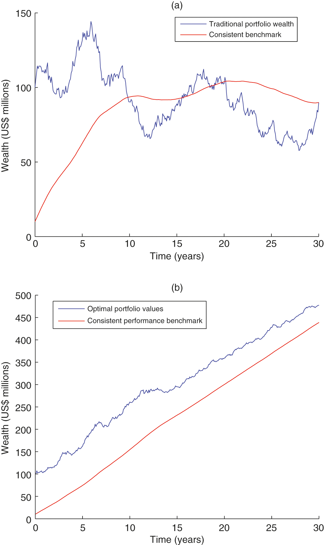
To begin, in Figure 1(a) we show one realization of the wealth scenario “traditional portfolio wealth”, following the traditional policy, as well as its corresponding moving average scenario “consistent benchmark”, . Here, is a weighted average of the historical wealth records . Evidently, the traditional portfolio wealth has a high likelihood of falling below the consistent substance. In other words, the consistent performance constraint is not satisfied.
By contrast, Figure 1(b) depicts portfolio wealth in a generic realization following a CPS. A major benefit of the CPS is the upward trend of its wealth path because it is supported by an upward substance. Indeed, Figure 1(b) demonstrates that the substance is always increasing under the CPS. Because of this increase, wealth exhibits an upward trend. Moreover, despite the increase or decrease of the wealth scenario, its total return is always bounded below by a positive number. Hence, the return is guaranteed and the capital is protected.


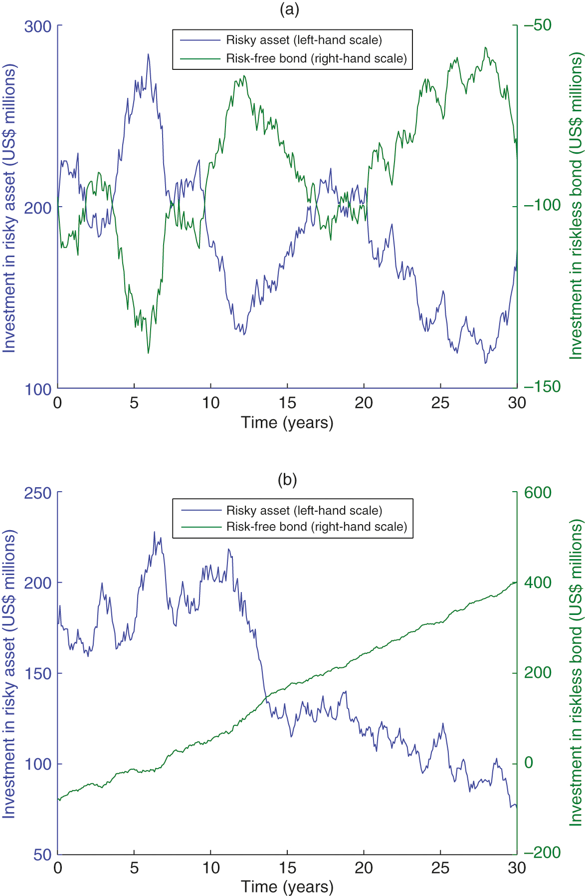
To examine this CPS closely, Figure 2 depicts the trading positions in one realization of the wealth scenario under these two trading strategies. Figure 2(a) shows that the traditional strategy is a relatively aggregative strategy, as it involves borrowing heavily to invest in the risky asset, despite the decline or increase of portfolio wealth. More precisely, the investor keeps borrowing and investing in the risky asset, even though the portfolio starts to decline six years later. This borrowing hits its peak at around six years, but the traditional strategy still recommends continuous borrowing, which it invests in the risky asset. The CPS, however, is rather conservative, striking a more appropriate balance between the risky and the risk-free asset. We show the trading positions of the CPS in Figure 2(b) using the same business situation as in Figure 2(a). Following the CPS, the investor stops borrowing at the early stages of the investment horizon and then gradually reduces their investment in the risky asset. As a result, the risk-free positions accumulate a large capital cushion and, at the same time, the risky positions contribute stable returns.
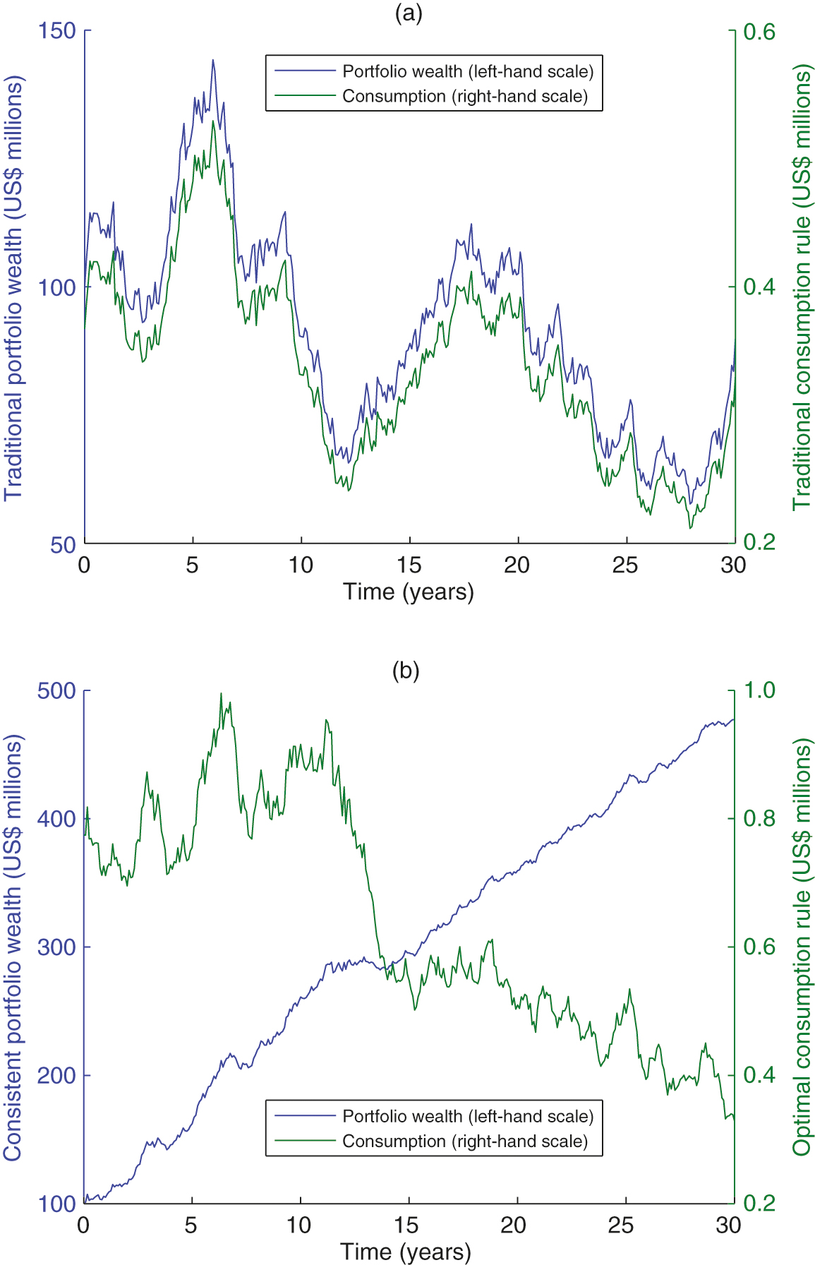
We now move to the consumption or spending rule. The dynamic consumption rules in both strategies (traditional and CPS) are displayed in the two panels of Figure 3. The consumption in Figure 3(a), under the traditional strategy, is always a constant proportion of portfolio wealth by construction. However, as shown in Figure 3(b), the dynamics of portfolio wealth and the consumption rule under a CPS have starkly different shapes, since the investor consumes only a constant proportion of the capital cushion instead of the wealth itself. Therefore, an upward trend in portfolio wealth does not always mean the investor is consuming more. Moreover, less consumption ensures more investment in the risk-free asset so as to add more of a capital cushion. Having a capital cushion is vital in the CPS in order to hedge against future uncertainties, withstand future losses and obtain stable wealth growth.


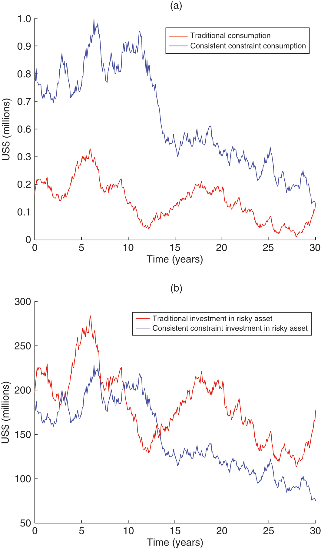
Finally, Figure 4 demonstrates the consumption and risky investment positions of both the traditional strategy and the CPS together, under the same realization of the asset return. Figure 4(a) shows the clear difference in consumption between these two strategies. It is worth noting that the CPS does not always sacrifice investors’ consumption because of its stable return. In Figure 4(a), the CPS actually provides a (relatively) higher spending rate than the traditional strategy. Again, this phenomenon comes from the stable cashflows generated by the risk-free position of the CPS; the tradition strategy, however, is relatively aggressive, so the cashflows generated from its risk-free position might be insufficient to support a large consumption demand.
Figure 4(b) shows the difference in risky positions of these two strategies. Under the traditional strategy, the investor shorts a large amount of risk-free bonds and invests what they borrow in a risky asset. The CPS, meanwhile, always keeps a capital cushion and invests in a risk-free asset to generate a steady stream of cashflows, thus building a less risky position than the traditional strategy.
3.2 Portfolio performance
We now demonstrate some more potentially attractive features of the CPS – its low volatility and high Sharpe ratio – by studying its expected return, standard deviation, Sharpe ratio and leverage ratio.
| (a) % | ||||
| Standard | ||||
| Expected | deviation | Sharpe | ||
| return (%) | (%) | ratio | Leverage | |
| 0.005 | 2.0168 | 0.3105 | 0.6434 | 0.7743 |
| 0.010 | 2.0166 | 0.2607 | 0.7656 | 0.6481 |
| 0.015 | 2.0165 | 0.2248 | 0.8875 | 0.5574 |
| 0.020 | 2.0165 | 0.1974 | 1.0103 | 0.4889 |
| 0.025 | 2.0164 | 0.1763 | 1.1316 | 0.4355 |
| 0.030 | 2.0164 | 0.1591 | 1.2533 | 0.3925 |
| 0.035 | 2.0164 | 0.1450 | 1.3754 | 0.3573 |
| 0.040 | 2.0164 | 0.1331 | 1.4975 | 0.3279 |
| 0.045 | 2.0163 | 0.1231 | 1.6196 | 0.3030 |
| 0.050 | 2.0163 | 0.1144 | 1.7417 | 0.2815 |
| (b) % | ||||
| Standard | ||||
| Expected | deviation | Sharpe | ||
| return (%) | (%) | ratio | Leverage | |
| 0.005 | 2.0191 | 0.7439 | 0.6978 | 2.0118 |
| 0.010 | 2.0182 | 0.6248 | 0.8295 | 1.6826 |
| 0.015 | 2.0178 | 0.5385 | 0.9613 | 1.4462 |
| 0.020 | 2.0174 | 0.4731 | 1.0936 | 1.2681 |
| 0.025 | 2.0172 | 0.4219 | 1.2258 | 1.1292 |
| 0.030 | 2.0170 | 0.3807 | 1.3580 | 1.0177 |
| 0.035 | 2.0169 | 0.3467 | 1.4908 | 0.9263 |
| 0.040 | 2.0168 | 0.3185 | 1.6227 | 0.8500 |
| 0.045 | 2.0167 | 0.2944 | 1.7549 | 0.7853 |
| 0.050 | 2.0166 | 0.2738 | 1.8871 | 0.7297 |
Table 1 reports the expected return, standard deviation and Sharpe ratio of the portfolio when the free parameter moves from 0.5% to 5%. The last column, “Leverage”, will be explained shortly. There are two different interest rate environments in Table 1: a relatively high interest rate environment, (panel (a)), and a relatively low interest rate environment, (panel (b)).
When , as shown in Table 1, the expected return is fairly stable, moving around 2.016% with different choices of the parameter . If we look at Table 1 more closely, the expected return decreases slightly as parameter increases. The intuition behind this is straightforward. A low value of parameter leads to a flat consistent performance substance curve, so the investor is able to invest in large risky positions and still meet the consistent performance constraint. Consequently, the expected return of the portfolio wealth decreases with respect to . Since the standard deviation of the return rate grows due to the increase in risky positions, increasing the parameter also ensures a decreasing standard deviation of the return.
Remarkably, the standard deviation of the return rate drops more significantly than the expected return rate does when the tuning parameter increases in the same way. As a consequence, the corresponding Sharpe ratio measure increases. The Sharpe ratio can be as large as 1.74 when is chosen as 5% (see Table 1).
Therefore, the proposed CPS generates a robust “low risk and better performance” trading strategy, particularly when the substance curve is fairly steep. If the interest rate drops to , the risky asset becomes more attractive and the Sharpe ratio is even higher for the same parameter . Overall, increasing parameter reduces both the expected return and the standard deviation but significantly increases the associated Sharpe ratio in different interest rate environments.
3.3 Leverage position
The amount invested in the risky asset is a constant proportion of the capital cushion. Thus, the portfolio weight of the total wealth in the risky asset is . If , then , so there is no short position in the risky asset and the risk-free asset. However, if the expected return of the risky asset is large enough, or if the volatility is sufficiently low, or if the investor is less risk averse, then the proportion can be greater than , implying a possible short position in the risky asset. Therefore, the weight can be greater than and the investor gains a leverage position by borrowing.
We explain under what conditions the leverage position exists on average, ie, , where denotes the expectation, and the associated probability distribution function of is given in Appendix A (available online). The last column in Table 1 reports the expected value of the leverage, , with respect to parameter for two different interest rate scenarios: and . As can be seen in Table 1, as increases, decreases regardless of the interest rate value. The intuition is the same as that behind our previous discussion. A smaller value of parameter means that the investor intends to have a larger position in the risky asset; therefore, increases. When the interest rate drops from to , the risky asset becomes more attractive, so becomes higher. The numerical result reported in Table 1 supports this.
4 Forward testing of CPS
In the last section, we implemented the CPS under the normal distribution assumption of a risky asset (index). The model parameters are calibrated using S&P 500 index data from 1983 to 2016. While there is a vast literature documenting the normality of market index returns (see, for instance, Malkiel 1998), we might also argue the opposite by citing a great number of empirical asset pricing studies, such as Lo and MacKinlay (1999) and Moskowitz et al (2012). In this regard, is the CPS too sensitive to the model assumption? Moreover, does the strategy display a robust consistent performance feature under walk-forward testing (Pardo 2008) or not?
To address this problem, we perform a forward (walk-forward) testing exercise of the CPS using historical data from the market index. For illustrative purposes, we make use of monthly data so that we are able to examine the performance over a long time period. Our objective is to demonstrate that the CPS offers similar insights in this exercise to those discussed above regarding the simulated scenarios in Section 3.

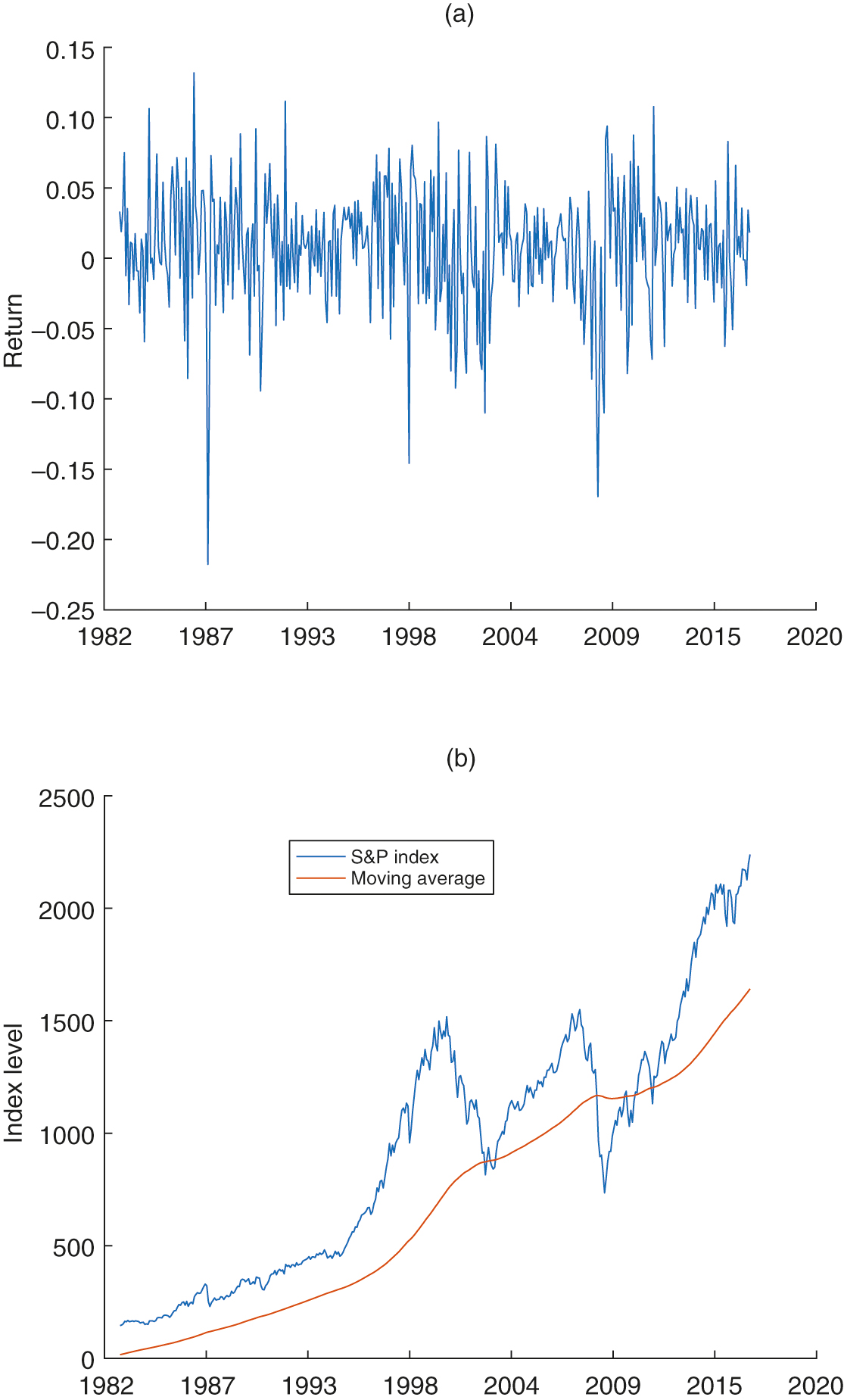
To start with, we show the monthly return data and the monthly level data of the S&P 500 for January 1983–December 2016 in Figure 5(a) and Figure 5(b), respectively. Indeed, the normality of the monthly return cannot always be guaranteed by the Kolmogorov–Smirnov test. The level of the S&P 500 is 145.3 on January 31, 1983 and 2238.8 on December 30, 2016. In general, the market displays an upward trend except in two very bad time periods – the 1999–2003 market meltdown and the 2008–9 financial crisis – and the market drops more than 40% during each of these time periods.

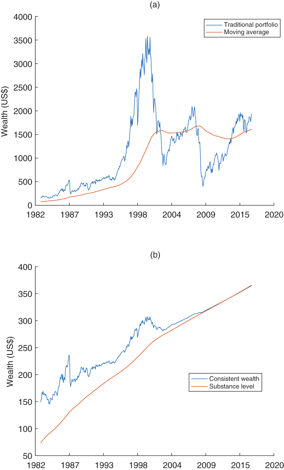
Next, we use the entire time period of historical data to examine the performance of the consistent strategy. In Figure 6(a), we implement the same traditional (Merton) strategy as in Section 3 and compute the corresponding moving average with the same parameters: and . We choose the initial substance level as . As shown, the traditional strategy is quite aggressive for the investor, with a risk-aversion parameter of 0.3, since they invest times their wealth into the index. The traditional portfolio offers a great performance from 1986 to 1999; but its performance from 1999 to 2016 is not so appealing, and not even as good as that of the index itself. As a result, the consistent performance constraint does not always hold. It is worth mentioning that , representing a fairly aggressive traditional strategy.
By contrast, we implement the CPS in Figure 6(b). The substance level is calculated with the same parameters as in Figure 6(a). As shown, the substance level clearly displays an upward trend, as the model predicts in Sections 2 and 3. The downward trend of the index itself affects the portfolio, but a large amount of the reserve can be used to smooth out the negative market movement, particularly during the time period covering the 2008–9 financial crisis. In consequence, the risk (volatility) of the CPS is much smaller than that of the traditional strategy.
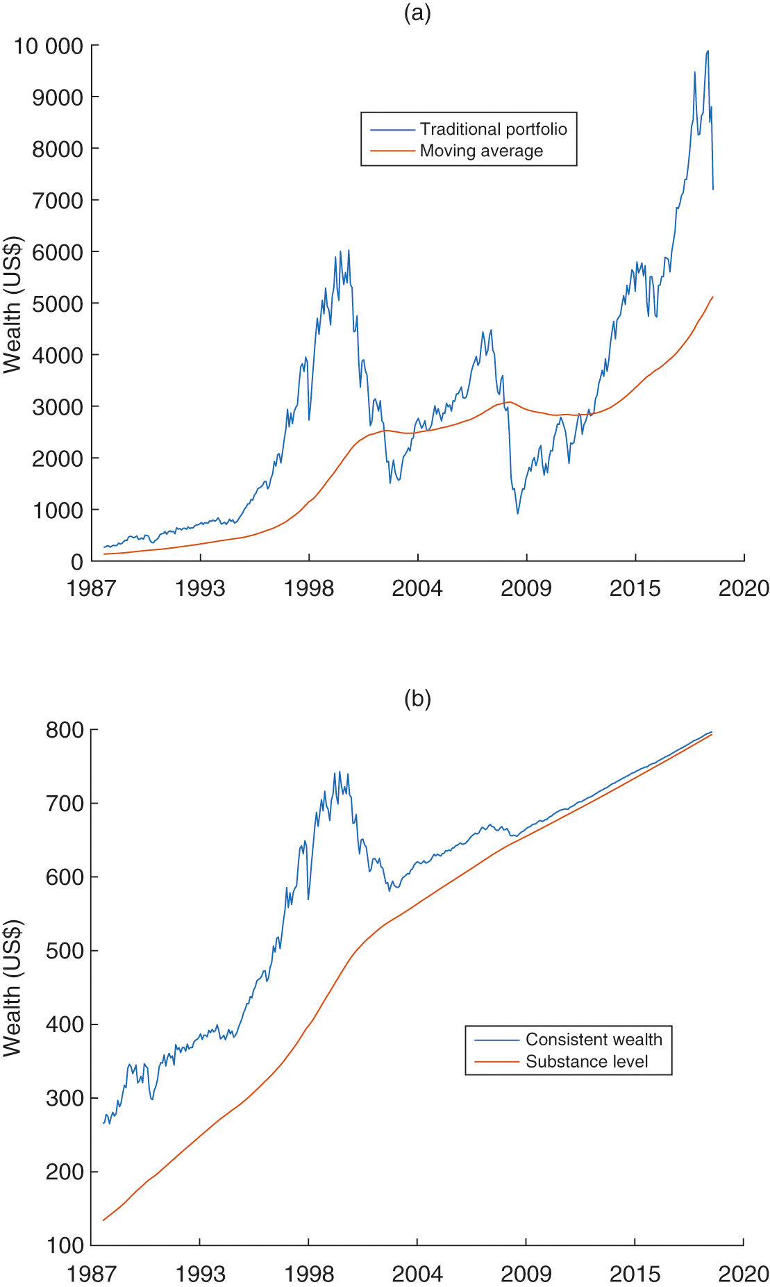
Since the dividend is often reinvested in the index, we start to make use of an equity index that has reinvested the dividend in our following discussions. Specifically, in our remaining forward-testing exercises, we use the S&P 500 total return index (SPXTR) from April 1988 to December 2018, which is available from Bloomberg.33 3 We also finish our walk-forward testing for the S&P index, and the main insights are similar. We thank the referee for a suggestion to focus on the SPXTR; other results for the S&P 500 index are available from the authors. In Figure 7(a), we show the traditional strategy and the corresponding moving average using historical SPXTR data from April 1988 to December 2018. The parameters to calculate the moving average are the same as in Figure 6. For the same historical data, we show the consistent strategy and the corresponding moving average in Figure 7(b). The initial substance level is . As shown, Figures 6 and 7 display very similar results for the consistent strategy regardless of whether SPX data or SPXTR data is used.

We now move on to the walk-forward testing of the CPS.44 4 We are grateful to an anonymous referee for a remarkable suggestion to make use of the walk-forward methodology to robustly test the proposed strategy.
4.1 Walk-forward testing
The main idea behind the walk-forward test is to divide our test data into a sequence of in-sample data and then to verify the strategy (system) by testing it forward in time on out-of-sample data. Unlike in backtesting, we can evaluate the strategy based on how well it performs using test data rather than the data on which it has been calibrated and optimized.
Due to the monthly return frequency, we use a relatively long time period for the sample window in our walk-forward testing exercise. More precisely, we consider three different situations. In the first, we make use of ten-year market data as our in-sample test data and choose the optimal parameter . In the second, we implement the consistent strategy on the next year and compare the outcome of the consistent strategy with the market index (out-of-sample testing data). This situation is termed “10–1” walk-forward testing. Similarly, we also consider “10–2” and “15–3” situations in our forward-testing exercise.
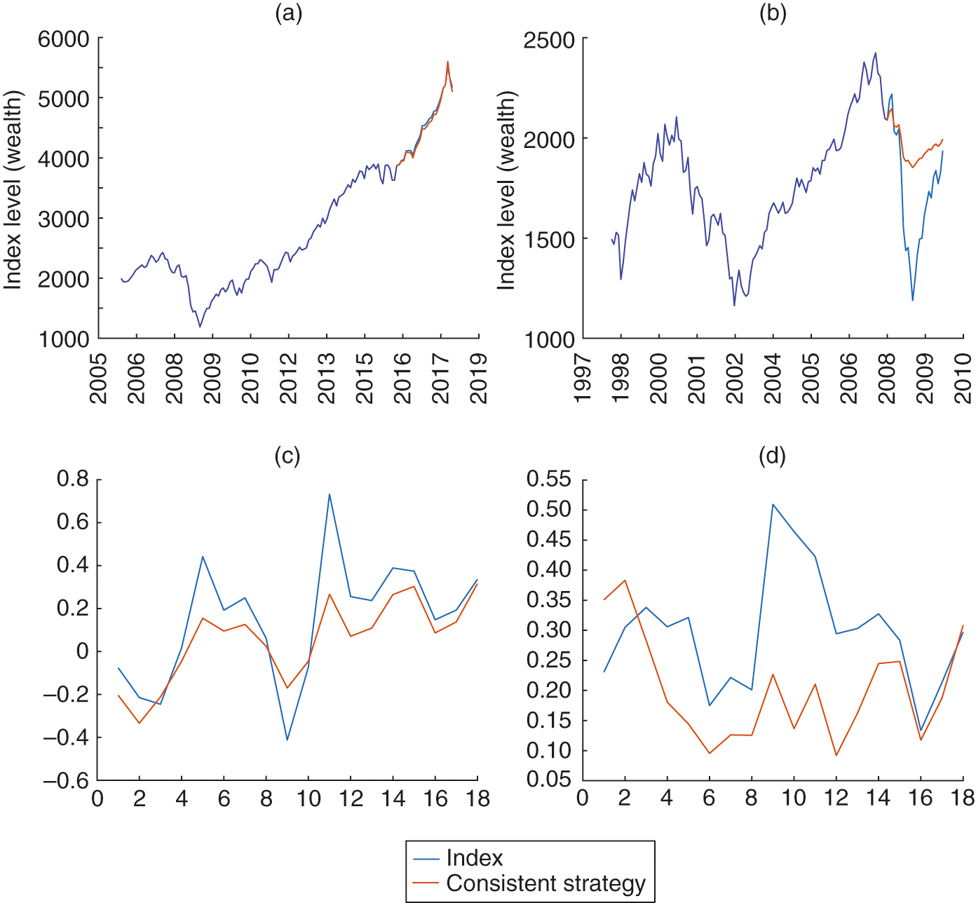
In the “10–1” walk-forward testing exercise, there are nineteen sequences of sample window in total. In each sample window, the market data of ten consecutive years is used as the in-sample data, and the following year is used to compare the strategy with the out-of-sample data. Figure 8(a) displays the results for June 2005 to May 2016. The time period June 2005 to May 2015 is the in-sample time period, while June 2015 to May 2016 is the out-of-sample time period. If we implemented the consistent strategy in 2015 using the calibrated parameter in the in-sample time series, the portfolio would be in line with the upward trend of the index. Its return is not as good as the index itself; however, the (consistent strategy) portfolio return in less volatile than the market index. Figure 8(b) displays the result of a downward market. In Figure 8(b), the in-sample time series is the monthly data from September 1997 to August 2007. It is well-known that the market enters a downward trend from mid-2007 until 2009. If we implemented the consistent strategy in 2007, the portfolio would still generate a negative return, but its performance would clearly be much better than the S&P market index for this year.

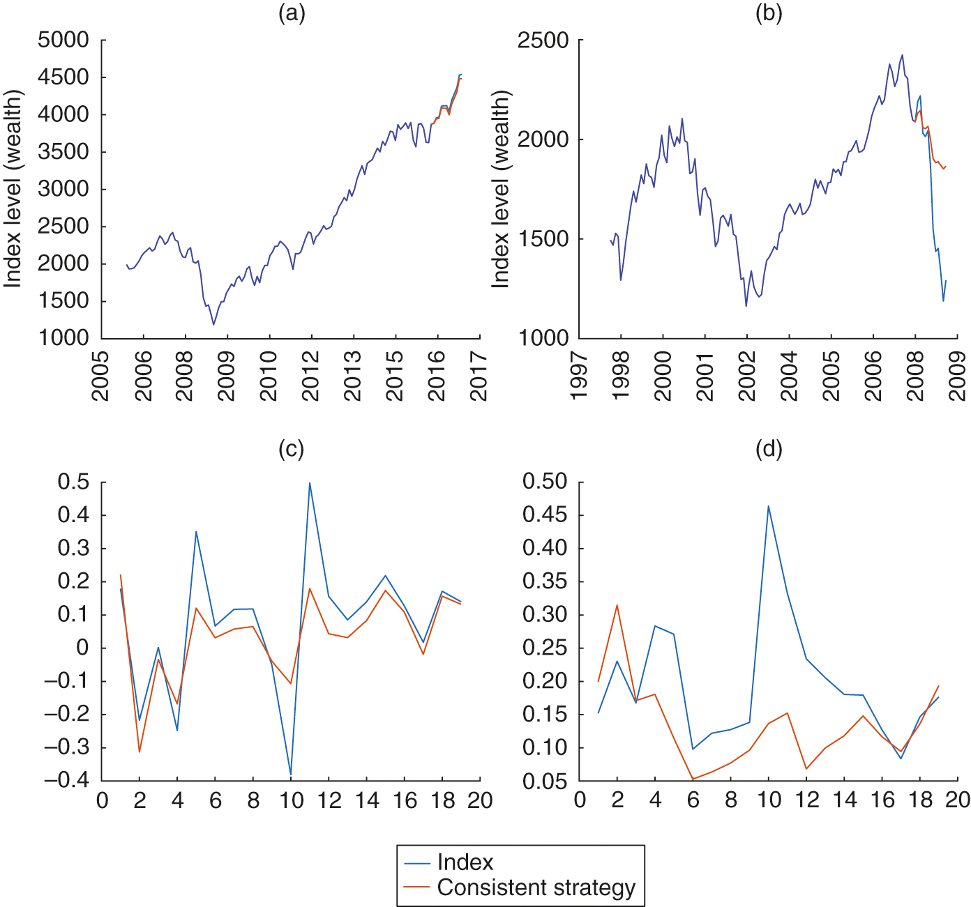
To be brief, we do not exhibit all nineteen sample windows (scenarios) tested using this “10–1” strategy; instead, we report the risk and return of the portfolio versus the index in the out-of-sample time period. Figure 8(c) displays the return in each sample window. As shown, the portfolio return is smaller than the index return in an upward market but larger than the index return in a downward market (for instance, in sample windows 4 and 10). We also report the risk of the consistent strategy. In each year, we calculate a relative (maximum) drawdown measure (the maximum loss from a peak during this particular time period, representing a percentage of the peak) for both the index and the consistent strategy’s portfolio. By its nature, the smaller the relative drawdown, the less risky the strategy. As shown in Figure 8(d), the consistent strategy generates a much smaller maximum drawdown measure than the index in the same out-of-sample time period except for in the first two sample windows.
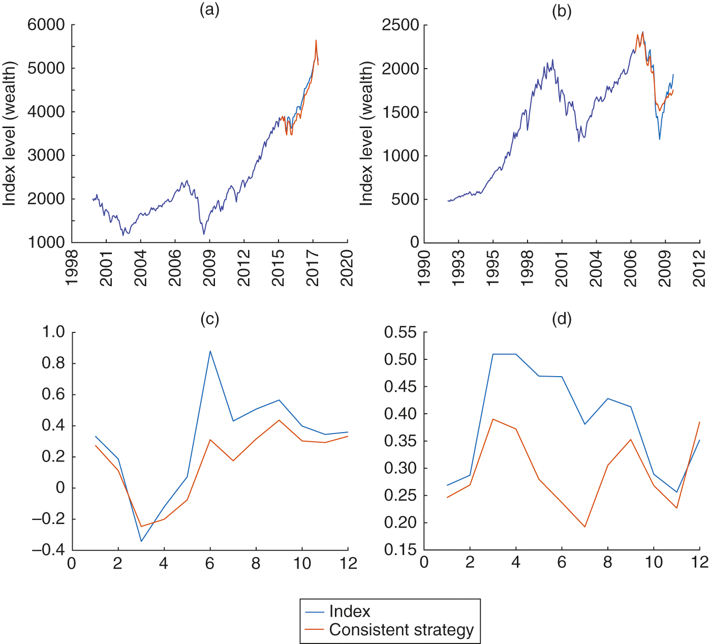
For the purposes of robustness, we further display the walk-forward testing result for “10–2” and “15–3” in Figures 9 and 10, respectively. In both figures, part (a) displays the consistent strategy’s portfolio versus the index in an upward trend scenario, while part (b) illustrates this comparison in a downward trend scenario. We also report the return and drawdown risk in parts (c) and (d), respectively, for each situation. Overall, the walk-forward testing exercise of the CPS shows similar insights as presented in both the model and the simulated scenarios in Section 3. The CPS could be appealing to conservative investors whose targets are stable performance, low risk and a consistent strategy, or when the market itself drops significantly. However, its conservative features could miss great opportunities in an expanding economy, as was the case for 1983–99.
It is worth mentioning that the implementation of the consistent strategy is sufficiently flexible to construct the substance level. For instance, both the moving average window and the parameters should be considered in its implementation system. Exactly how to balance a consistent performance with risk taking is clearly an ongoing research topic in asset management.


4.2 The effect of risk aversion
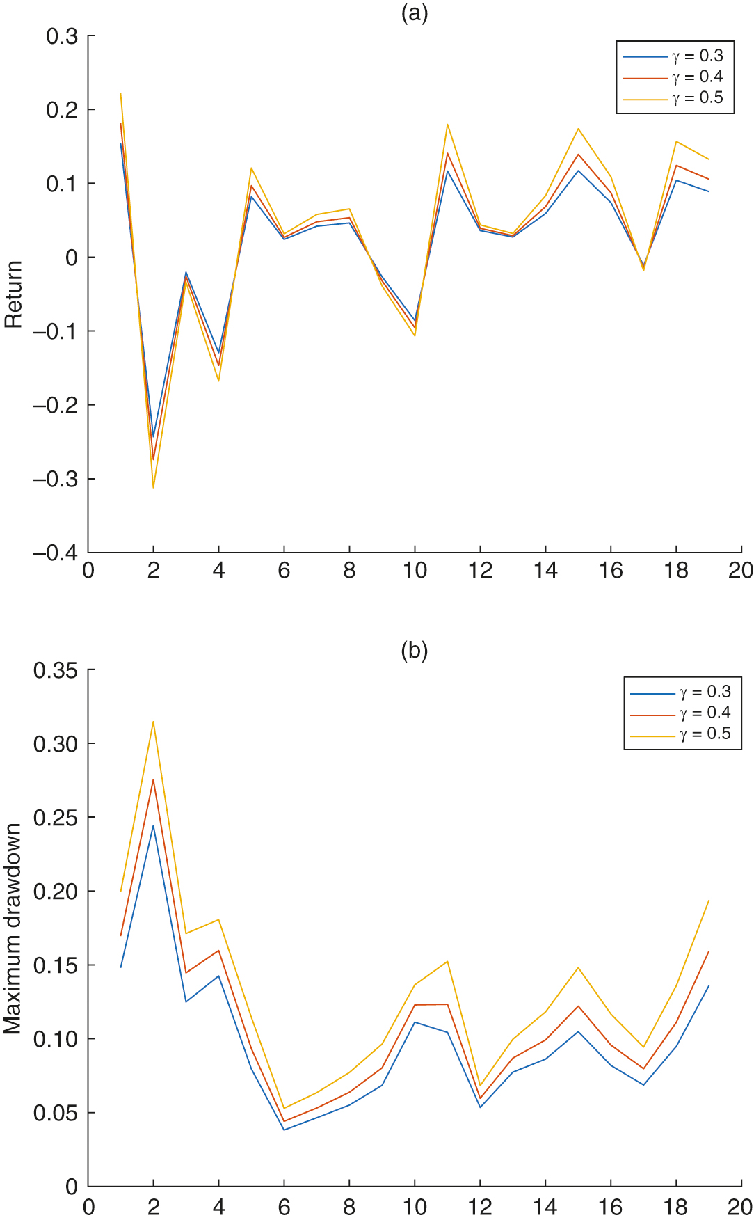
As an investor becomes more risk averse, they require more of a capital cushion, reducing the amount of wealth in the CPS. Moreover, when the investor is less risk averse, they need to invest more in risky assets and less in risk-free bonds.55 5 In our setting, for and is the constant relative risk-aversion parameter. Thus, a smaller represents a more risk-averse investor.
We continue the walk-forward testing exercise for different parameters using the “10–1” in- and out-of-sample market data. Figure 11 reports the risk–return of the consistent strategy in the test data for nineteen years when , respectively. Specifically, Figure 11(a) shows that the return of the consistent strategy for a more risk-averse investor is “smaller” than that of a less risk-averse agent in a strong market; however, it boasts a better return in a weak market when all returns are negative. Figure 11(b) displays the maximum drawdown measures following the CPS for these investors. Evidently, and robustly, the more risk averse the investor, the less risky the consistent strategy. While the consistent strategy may appeal to conservative investors, Figure 11 shows that the consistent feature of the strategy becomes more attractive the more risk averse the investor.

5 Conclusion
We introduce a CPS that generates consistently growing portfolio wealth. An attractive feature of this CPS is the upward trend in portfolio wealth it exhibits, regardless of whether good or bad times are affecting the underlying equity market. Another distinctive feature of the CPS is its low volatility and high Sharpe ratio. These capital-protection and low-volatility features should make the CPS appealing to some types of investors such as pension or endowment funds.
Declaration of interest
The authors report no conflicts of interest. The authors alone are responsible for the content and writing of the paper.
Acknowledgements
The authors are grateful for the comments and suggestions from the anonymous referees that have improved this paper. The authors report no conflicts of interest. The authors alone are responsible for the content and writing of the paper.
References
- Black, F., and Perold, A. (1992). Theory of constant proportion portfolio insurance. Journal of Economic Dynamics and Control 16, 403–426 (https://doi.org/10.1016/0165-1889(92)90043-E).
- Bogle, J. (1999). Common Sense on Mutual Funds: New Imperatives for the Intelligent Investor. Wiley.
- Chen, X., and Tian, W. (2014). Optimal portfolio choice and consistent performance. Decisions in Economics and Finance 37, 453–474 (https://doi.org/10.1007/s10203-013-0154-x).
- Constantinides, G. (1990). Habit formation: a resolution of the equity premium puzzle. Journal of Political Economy 98, 519–543 (https://doi.org/10.1086/261693).
- Dybvig, P. (1995). Dusenberry’s ratcheting of consumption: optimal dynamic consumption and investment given intolerance for any decline in standard of living. Review of Economic Studies 62, 287–313 (https://doi.org/10.2307/2297806).
- Dybvig, P. (1999). Using asset allocation to protect spending. Financial Analysis Journal January/February, 49–62 (https://doi.org/10.2469/faj.v55.n1.2241).
- Grossman, S., and Zhou, Z. (1993). Optimal investment strategies for controlling drawdowns. Mathematical Finance 3, 241–276 (https://doi.org/10.1111/j.1467-9965.1993.tb00044.x).
- Lo, A., and MacKinlay, C. (1999). A Non-Random Walk Down Wall Street. Princeton University Press.
- Malkiel, B. (1998). A Random Walk Down Wall Street. W. W. Norton & Company.
- Maymin, P., and Maymin, Z. (2011). Constructing the best trading strategy: a new general framework. The Journal of Investment Strategies 1, 1–22 (https://doi.org/10.21314/JOIS.2011.076).
- Merton, R. (1971). Optimum consumption and portfolio rules in a continuous-time model. Journal of Economic Theory 3, 373–413 (https://doi.org/10.1016/0022-0531(71)90038-X).
- Moskowitz, T., Ooi, Y. H., and Pedersen, L. H. (2012). Time series momentum. Journal of Financial Economics 104, 228–250 (https://doi.org/10.1016/j.jfineco.2011.11.003).
- Murphy, J. (1999). Technical Analysis of the Financial Markets: A Comprehensive Guide to Trading Methods and Applications. New York Institute of Finance.
- Pardo, R. (2008). The Evaluation and Optimization of Trading Strategies, 2nd edn. Wiley.
- Zhu, Y., and Zhou, G. (2009). Technical analysis: an asset allocation perspective on the use of moving averages. Journal of Financial Economics 92, 519–544 (https://doi.org/10.1016/j.jfineco.2008.07.002).
Only users who have a paid subscription or are part of a corporate subscription are able to print or copy content.
To access these options, along with all other subscription benefits, please contact info@risk.net or view our subscription options here: http://subscriptions.risk.net/subscribe
You are currently unable to print this content. Please contact info@risk.net to find out more.
You are currently unable to copy this content. Please contact info@risk.net to find out more.
Copyright Infopro Digital Limited. All rights reserved.
As outlined in our terms and conditions, https://www.infopro-digital.com/terms-and-conditions/subscriptions/ (point 2.4), printing is limited to a single copy.
If you would like to purchase additional rights please email info@risk.net
Copyright Infopro Digital Limited. All rights reserved.
You may share this content using our article tools. As outlined in our terms and conditions, https://www.infopro-digital.com/terms-and-conditions/subscriptions/ (clause 2.4), an Authorised User may only make one copy of the materials for their own personal use. You must also comply with the restrictions in clause 2.5.
If you would like to purchase additional rights please email info@risk.net