This article was paid for by a contributing third party.More Information.

Multiyear analysis

A well-known technology for modelling simulated liability cash flows is the Least Squares Monte Carlo (LSMC) method. Changes in the value of liabilities are modelled to follow an interpolation function, where explanatory variables include claims and behavioural and capital market-related factors. A typical choice in life insurance is to use mortality, lapses and capital market prices and volatilities as proxy variables. When we combine the proxy model with asset valuations, we have a set-up for asset/liability management. But, to make that work for the own risk and solvency assessment (Orsa) process, we need to alter the process for multiyear analysis and, in doing this, we face a number of challenges:
- While a proxy model is a time-zero model for market-consistent values, Orsa processes work with real-world market simulations.
- In multiyear analysis, there is not a common starting point for many simulation paths, but there are many simulation paths that have only a single simulated future.
- To extend a liability proxy model for multiyear analysis, all events that have taken place in each of the simulation paths need to be be taken into account.
- An estimate for the solvency capital requirement (SCR) for all simulation paths and time steps for given simulated events would need to be made.
- There is a need to value all assets along all simulation paths, and time steps according to prevailing simulation circumstances.
There are a number of approaches to dealing with these challenges. The Model IT approach can be characterised by the following steps:
We use stressed market-consistent simulations as a basis for a proxy model to ensure that our proxy model is based on interpolation rather than extrapolation. The simulation continues by applying the proxy model for liabilities and applying real-world simulations for everything else.
- We enrich our proxy model with memory. We collect information into state variables and have them as part of our proxy model, like claims and capital flows.
- To estimate standard SCR, we include as many SCR shock factors as we can in our proxy model. We then use the proxy model to produce SCR shock effects.
- For those SCR shocks that cannot be included in the proxy model, we have implemented a linear model based on other state variables.
- In the final step, we apply full valuation formulas for all assets. Bonds are priced against yield curves and other assets against relevant market variables such as stock indexes and real estate price indexes.
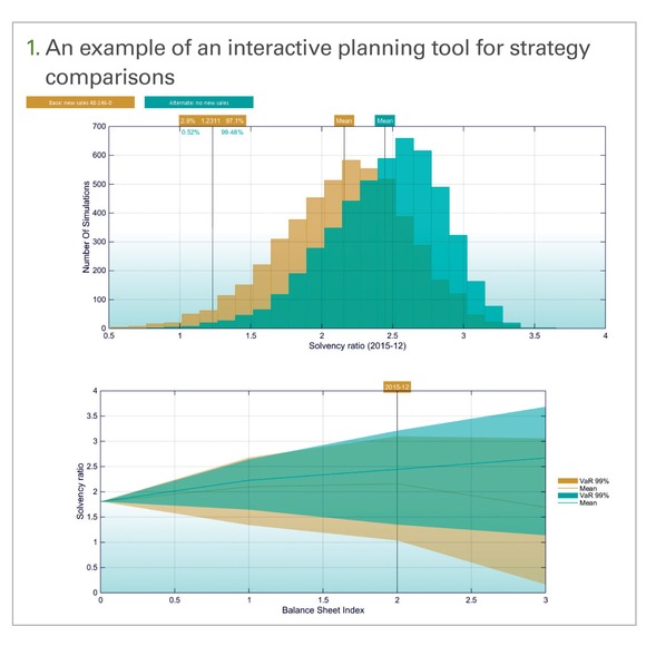
Once we have these properties available, we are ready to proceed with Or analysis. With a multiyear liability proxy and a full, step-by-step valuation of assets, we can simultaneously examine both sides of the balance sheet and apply complex decision-making rules and client behaviour. In our multiyear Orsa model, it is easy to plan and compare strategy options, not only by measuring averages but also by measuring probabilities and probability distributions, as illustrated here in figure 1.

The price invested in development time is rewarded by the accuracy and comprehensiveness of the results. This results in a single consistent model and technology base to support standard Orsa requirements and for all business decision-making needs.
Download/read the article in PDF format
Sponsored content
Copyright Infopro Digital Limited. All rights reserved.
As outlined in our terms and conditions, https://www.infopro-digital.com/terms-and-conditions/subscriptions/ (point 2.4), printing is limited to a single copy.
If you would like to purchase additional rights please email info@risk.net
Copyright Infopro Digital Limited. All rights reserved.
You may share this content using our article tools. As outlined in our terms and conditions, https://www.infopro-digital.com/terms-and-conditions/subscriptions/ (clause 2.4), an Authorised User may only make one copy of the materials for their own personal use. You must also comply with the restrictions in clause 2.5.
If you would like to purchase additional rights please email info@risk.net