Semianalytical pricing and hedging of fixed and indexed energy swing contracts

Benjamin Berger, Martin Dietrich, Rainer Döttling, Pascal Heider and Klaus Spanderen

Abstract

Typical natural gas derivative contracts in the wholesale market contain several multifaceted flexibilities, which protect buyers from fluctuations in price and demand. We will focus on fair market valuation as well as hedging of the most common type of these contracts: swing options. We follow the ideas of a seminal 2004 article by Keppo and decompose swing contracts into tradable products. While Keppo considers only forwards and call options to decompose the flexibility in a fixed swing contract, we add time-spread optionality. Moreover, we extend Keppo’s decomposition approach to cover indexed swing contracts. To this end, we introduce a simple spot price model and use reasonable approximations to account for the indexed swing’s inherent Asian optionality. In contrast to standard least- square Monte Carlo valuation techniques, which are limited by increasing memory constraints, our heuristic valuation approach allows for an arbitrary number of period volume constraints of the swing contract. Further, our approach can deal with 100% take-or-pay contracts, which are typically not covered by Keppo-like valuation methods, and we will derive and backtest analytical approximations for the swing contract’s Greeks.
 

Download PDF

Introduction

1 Introduction

Typically, the exact required volumes of commodity supply contracts are not known by the time the deal concludes, and the buyer of the commodity volume requests the additional flexibility to take more (or less) volume than initially assumed. This might be due to changing market environments (eg, a producer of aluminum might need to increase power consumption due to an increase in demand), due to weather influences (eg, a gas wholesaler might need fewer gas volumes to distribute, due to an extraordinary warm winter season), or due to other market disturbances from the expected normal (eg, a decline in the world economy).

To get the required flexibility, the buyer can enter into a swing contract. This contract gives the holder the right to nominate certain volumes for a fixed price (fixed-price swings) in a certain period of time. For each period, the buyer and seller of the swing contract agree on a minimum and maximum volume, and the buyer can nominate volumes as long as these bounds are kept. These periods might be overlapping, and typically there is a total minimum and maximum constraint over the total lifetime of the contract. In this type of swing contract, the commodity price is agreed upon at the time of the deal conclusion.

Due to its lower price risk, another commonly used instrument is the indexed swing contract. In this type of contract the commodity price is indexed to a certain price tracker, and therefore it is fixed only after the conclusion of the contract.

In this paper, we focus on month-ahead indexed swing contracts, which means that the contract’s strike for each delivery month is tied to a price tracker. The price tracker is obtained by averaging the daily settled month-ahead forward product prices for each day within the month prior to delivery. As in the fixed-price case, additional constraints might be applied to each of the monthly delivery periods and the contract’s total delivery period.

Valuation methods for swing contracts have been discussed in several places in the literature (Wilhelm and Winter 2008; Carmona and Touzi 2008; Broadie and Glasserman 2004; Dahlgren 2005; Jaillet et al 2004) with a particular focus on stochastic optimal control methods (Longstaff and Schwartz 2001; Lari-Lavassani et al 2001; Barrera-Esteve et al 2006). In any case, for the valuation of the swing contract, it is usually assumed that the buyer will exercise their swing rights in a market optimal way. In this paper, we follow the ideas outlined in Keppo (2004) and optimally but statically decompose the swing contract into tradable products. While Keppo (2004) considers only forwards and call options to decompose the flexibility in a fixed swing contract, we add time-spread optionality.

Further, we extend Keppo’s decomposition approach to cover indexed swing contracts. To this end, we introduce a simple lognormal spot price model and use reasonable approximations to account for the indexed swing’s inherent Asian and time-spread optionalities (interchanging spot volatility from one month to the other). In conjunction with our monthly geometric Brownian motion (GBM) forward model, this is sufficiently flexible to model the seasonalities of the forward curve as well as the volatility surface. At the same time, the model allows (approximative) analytical expressions for the option values.

While we have chosen this particular market model, our extension of Keppo’s valuation framework can be applied more generally to any other model, eg, Heston-like or other non-Gaussian models that provide reasonable values for the optionalities to be priced. Analogously, we have chosen one particular index tracker, ie, the most commonly traded month-ahead index, whereas any other tracking index could be applied. If in the ideal case all decomposition products are liquidly traded and prices can be observed in the market, our swing valuation method becomes “model free”.

Our heuristic swing valuation approach allows an arbitrary number of period volume constraints, in contrast to standard least-square Monte Carlo (LSMC) valuation techniques, which are limited by increasing memory constraints. Further, our approach can deal with 100% take-or-pay contracts (ie, a swing contract with minimum total volume equal to the maximum total volume). This flexibility class has previously not been covered by Keppo-like valuation methods.

From a risk management and trading perspective, our decomposition approach has the advantage that valuation and hedging decisions can be based on tradable products. Therefore, we will discuss Greeks and sensitivities for our suggested decomposition. We will derive analytical approximations for Delta, which can be extended straightforwardly to cover Gamma and Vega.

Further, several common applications of a valuation model, such as backtesting of trading strategies, stress tests and scenario analysis, involve numerous repeated valuations. Considering the backtesting use case, for instance, the number of required valuations of net present value (NPV) and Greeks can easily exceed several hundred. Particularly for such involved calculations, our valuation methodology offers the advantage of being numerically very fast.

In the next section, we will set the notation and define the most general case of a swing option. In this setup, we will also discuss the swing constraints, which will later serve as linear optimization bounds. In Section 3, we will outline our underlying market model and a valuation model for the decomposition products of indexed swings. Numerical examples will be provided in Section 4.

2 Swing contracts and energy markets

In this section, we set the notation for this paper and give background. We will discuss contractual details of fixed and indexed swings and introduce Keppo’s decomposition approach with our extension.

Throughout the paper, we will adopt a time discretization in daily granularity, as this is best suited for our focus on gas markets. Of course, a finer or coarser granularity can be applied in the same manner. Each fixed and indexed swing contract must have a total (primary) delivery period, which we denote by

$${\mathrm{\Pi }}_1=\{t_1^1,\mathrm{\dots },t_{N_1}^1\}$$

and which consists of consecutive delivery days $t_1^1$ till $t_{N_1}^1$. Further, there might be $M-1$ additional constraint periods

$${\mathrm{\Pi }}_j=\{t_1^j,\mathrm{\dots },t_{N_j}^j\}\subset {\mathrm{\Pi }}_1$$

for $j=2,\mathrm{\dots },M$ with $t_i^j\in \{t_1^1,\mathrm{\dots },t_{N_1}^1\}$.

For each of the $j=1,\mathrm{\dots },M$ periods there is a minimum volume constraint ${\mathrm{\Pi }}_j{\text{CQ}}_{\min }$ and a maximum constraint ${\mathrm{\Pi }}_j{\text{CQ}}_{\max }$. Note that typical over-the-counter-traded swing contracts have an annual total delivery period (in which case we say ${\text{ACQ}}_{\min }$ and ${\text{ACQ}}_{\max }$) and constant daily constraints (${\text{DCQ}}_{\min }$ and ${\text{DCQ}}_{\max }$).

The valuation day will be denoted by $t_{*}$. We say that the swing contract is in delivery if $t_{*}\ge t_1^1$. If the swing is in delivery we denote by $a(t_i)$, $t_i\in {\mathrm{\Pi }}_1$, the nominated volume on day $t_i$ for all days with $t_i\le t_{*}$. To avoid cumbersome indexation we set all future volumes $a(t_i)=0$ for days $t_i>t_{*}$.

On the valuation day we assume that a daily granular forward curve of the considered commodity is available. We will denote by $F_i$ the forward price of the commodity for delivery on day $t_i$. Typically, this forward curve is constructed arbitrage-free from observable forward products.

2.1 Decomposition of energy swing contracts

In the fixed swing case, both parties agree on a (fixed) delivery price $K_i$ for each day $t_i$. Hence, if the buyer of the swing nominates on day $t_i$, they will receive the commodity and pay $K_i$ for each taken volume. Of course, the buyer can only nominate volumes such that all minimum and maximum constraints of this contract are not violated.

We will decompose the swing optionality into forward products, call options and time-spread options. The rationale behind this approach is that the contractual “minimal takes” induce a certain forward (minimum) profile, which the buyer is obligated to take, a set of days on which the buyer can choose whether or not to call additional volumes and the flexibility of the buyer to (freely) choose the time of a mandatory exercise. The assignment of forwards, call and swap rights must, however, satisfy the contractually agreed constraints in all exercise scenarios.

We note that this decomposition is only a lower bound of the full value of flexibility in the swing contract. For example, we decompose a contract in European-type vanilla options, although the flexibility in the swing contract is American type (the buyer can freely choose when to nominate the volume).

The canonical strategy to monetize this decomposition value is to create a portfolio with a long position in a swing contract and short positions in the decomposition products. From then on, the portfolio remains untouched in the sense that no additional options are added or removed. Finally, the swing option needs to be exercised to satisfy claims resulting from the short option positions. If the decomposition has been chosen wisely (ie, without breaching the swing constraints), all claims can be met with a corresponding exercise strategy. For completeness, it should be noted that in the case of a time-spread option expiring in-the-money, we also need to lock in the current spread by temporarily entering into a forward spread position. Generally, however, we call this strategy static, since in the time between initial portfolio setup and option expiry the positions are kept untouched regardless of any changes in the market.

This static trading strategy together with the market states at the expiry of each option determine the exercise strategy of the swing option. Broadly speaking, the swing is exercised whenever an option payoff needs to be paid. This exercise strategy eliminates the risk of any additional payments, but it is not necessarily “optimal” with respect to the highest swing payoff. The “optimality” strongly depends on the product constraints: for the edge case of a pure strip of options, we obviously yield the optimal exercise strategy. For 100% take-or-pay products (particularly short ones), the exercise strategy is far from optimal.

We will denote by $C_i$ the value (as of $t_{*}$) of a call option for one volume unit written on the forward delivering on day $t_i$ with strike $K_i$. Hence, the underlying of this option is the forward price $F_i$, and the payoff at maturity is $\max (F_i-K_i,0)$. The maturity of this option must be before delivery day $t_i$. Typically, these daily options are not traded separately in the market but are traded in a series of consecutive days (eg, for a month or a season). We will adopt a trader’s model to price a single daily option in Section 3.1.

Finally, we will denote by ${\mathrm{TS}}_{ij}$ the value of a time-spread option that will swap one volume unit of the forward delivering on day $t_i$ with one volume unit of the forward delivering on day $t_j$ at a strike level of $K_i-K_j$. Hence, the option’s payoff at maturity is given by $\max (F_i-F_j-(K_i-K_j),0)$. The maturity of this option occurs before $\min (t_i,t_j)$.

For each day $t_i\in {\mathrm{\Pi }}_1$, we will assign $f(t_i)$ forwards delivering on day $t_i$ with value $F_i$; $c(t_i)$ options on the forward of day $t_i$ with value $C_i$; and $\mathrm{ts}(t_i,t_j)$ time-spread options swapping forward on day $t_i$ with forward on day $t_j$ ($t_j\in {\mathrm{\Pi }}_1$) with value ${\mathrm{TS}}_{ij}$. We approximate the value $V$ of the swing contract by the value of the resulting hedge position. Hence, we get

$$V:=\max \sum _{t_i\in {\mathrm{\Pi }}_1}\left(f(t_i)(F_i-K_i)+c(t_i)C_i+\sum _{t_j\in {\mathrm{\Pi }}_1}\mathrm{ts}(t_i,t_j){\mathrm{TS}}_{ij}\right).$$

(2.1)

The maximum is taken over all admissible choices of the replicating portfolio $f(t_i)$, $c(t_i)$ and $\mathrm{ts}(t_i,t_j)$. Naturally, this means that the replicating portfolio must satisfy all period constraints in any circumstances, ie, any contingent claim resulting from the issued call and time-spread options should be grantable by executing the respective swing option accordingly.

This induces three constraints on the optimization problem in (2.1). First, to satisfy the minimum period constraint, we must have, for all periods $j=1,\mathrm{\dots },M$,

$$\sum _{t_i\in {\mathrm{\Pi }}_j^{*}}\left(f(t_i)-\sum _{t_k\in {({\mathrm{\Pi }}_1\setminus {\mathrm{\Pi }}_j)}^{*}}(\mathrm{ts}(t_k,t_i))\right)+\sum _{t_i\in {\mathrm{\Pi }}_j}a(t_i)\ge {\mathrm{\Pi }}_j{\text{CQ}}_{\min }.$$

(2.2)

The first term in the sum is due to the entered forward contracts. The second term, which sums the volumes of time-spread options, counts only if volume is potentially flowing out of the period ${\mathrm{\Pi }}_j$, while volumes potentially flowing into ${\mathrm{\Pi }}_j$ are neglected. This accounts for the fact that whether time-spread options are exercised or not is still subject to uncertainty. Therefore, the constraint is designed such that, even in the most unfavorable case with respect to exercised volumes within ${\mathrm{\Pi }}_j$, the swing contract constraints are still not breached. “Most unfavorable” in this context means that all outflowing time spreads are exercised but no inflowing time spreads are exercised, ie, the least possible volume is exercised within ${\mathrm{\Pi }}_j$. The last term counts the purchased volumes if valuation day $t_{*}$ is within the constraint period. The star notation on the index set indicates that only the $t_i\in {\mathrm{\Pi }}_j$ for which $t_i>t_{*}$ are admissible in the summation, ie, days that are in the future as seen from valuation day $t_{*}$.

To satisfy the maximum period constraints, we must have, for all $j=1,\mathrm{\dots },M$,

$$\sum _{t_i\in {\mathrm{\Pi }}_j^{*}}\left(f(t_i)+c(t_i)+\sum _{t_k\in {({\mathrm{\Pi }}_1\setminus {\mathrm{\Pi }}_j)}^{*}}(\mathrm{ts}(t_i,t_k))\right)+\sum _{t_i\in {\mathrm{\Pi }}_j}a(t_i)\le {\mathrm{\Pi }}_j{\text{CQ}}_{\max }.$$

(2.3)

In analogy to the minimum constraint, (2.2), we again face the problem of uncertain exercise volumes and thus require the most unfavorable exercise conditions to still preserve the constraints. In contrast to (2.2), here the most unfavorable case refers to the largest possible amount of exercised volumes within ${\mathrm{\Pi }}_j$. Accordingly, all futures (first term), all call options (second term) and all volume-adding time-spread options (third term) are taken into account, while all volume-extracting time-spread options are neglected.

Finally, as the swing contract only allows volume to be drawn but not pushed, we have to make sure that there is no net short position in the decomposition portfolio for each delivery day. Hence, we must have

$$\forall t_i\in {\mathrm{\Pi }}_1,f(t_i)-\sum _{t_j\in {\mathrm{\Pi }}_1}\mathrm{ts}(t_j,t_i)\ge 0.$$

(2.4)

Equations (2.1)–(2.4) together form a constrained optimization problem that can be solved by using standard numerical techniques.

The optimization problem is presented in the smallest granularity (here, daily) and is fully general. However, for practical applications it might be useful to consider a certain set of (allowed) call options and time-spread options. In particular, time-spread options are less liquidly traded, and typically we can only swap full months with each other. To account for this, we will generalize the above approach as follows.

In the rest of this section, we will denote by $F_i$, $i=1,\mathrm{\dots },n_{\mathrm{F}}$, the future prices for a product with delivery in the set $I_i^{\mathrm{F}}$:

$$F_i:=F_{I_i^{\mathrm{F}}}:=\frac{1}{|I_i^{\mathrm{F}}|}\sum _{t\in I_i^{\mathrm{F}}}F(t),$$

where $I_i^{\mathrm{F}}\subseteq {\mathrm{\Pi }}_1$ is a subset of the swing delivery dates. Note that the forward is written on one unit of volume for the delivery dates $I_i^{\mathrm{F}}$, and the volume is distributed equally on each day of $I_i^{\mathrm{F}}$. Typically, $I_i^{\mathrm{F}}$ relates to a certain day (as before), a month or a season.

Correspondingly, we will denote by $C_i$, $i=1,\mathrm{\dots },n_{\mathrm{C}}$, the call option prices for an option that is written on the future price for the delivery period $I_i^{\mathrm{C}}$. While it seems useful in applications, there is in general no need for the index sets $I_i^{\mathrm{C}}$ and $I_i^{\mathrm{F}}$ to coincide.

Further, we will denote by ${\mathrm{TS}}_{ij}$, $i,j=1,\mathrm{\dots },n_{\mathrm{TS}}$, the value of a time-spread option that swaps the forward $F_{I_i^{\mathrm{L}}}$ (long leg) defined by index set $I_i^{\mathrm{L}}$ and the forward $F_{I_j^{\mathrm{S}}}$ (short leg) defined by $I_j^{\mathrm{S}}$. Note that the time-spread option will swap one volume unit distributed equally in $I_i^{\mathrm{S}}$ to one volume unit distributed in $I_j^{\mathrm{L}}$.

Now, we can formulate (2.1)–(2.4) in the new setting. We will approximate the swing value by $f_i$ forward contracts with value $F_i-K_i$, $c_i$ call options with value $C_i$ and ${\mathrm{ts}}_{ij}$ time-spread options with value ${\mathrm{TS}}_{ij}$:

$$V:=\max \left[\sum _{i=1}^{n_{\mathrm{F}}}{f}_i(F_i-K_i)+\sum _{i=1}^{n_{\mathrm{C}}}{c}_i{C}_i+\sum _{i=1,j=1}^{n_{\mathrm{TS}}}{\mathrm{ts}}_{ij}{\mathrm{TS}}_{ij}\right].$$

(2.5)

The reformulation of the constraints (2.2)–(2.4) in this setup is slightly more complicated: for each product, the underlying index set ($I_i^{\mathrm{F}}$, $I_i^{\mathrm{C}}$, $I_i^{\mathrm{L}}$ or $I_i^{\mathrm{S}}$) might be partly outside the constraints period ${\mathrm{\Pi }}_j$, and therefore only parts of the volumes are relevant for the constraint $j$. First, we look at futures and call options: to account for the interference of the index sets and constraint periods, volumes are reduced by the fraction of the index set that is inside the constraint period, ie, for futures and calls we multiply by $|I_k^{\mathrm{F}}\cap {\mathrm{\Pi }}_j|/|l_k^{\mathrm{F}}|$ and $|I_k^{\mathrm{C}}\cap {\mathrm{\Pi }}_j|/|l_k^{\mathrm{C}}|$, respectively.

Figure 1: Influx and outflux of a time-spread call option.

Moreover, for each time-spread option ${\mathrm{TS}}_{kl}$, we have to determine its net volume outflux from the constraint period ${\mathrm{\Pi }}_j$. As illustrated in Figure 1, the net outflux reads

$$\frac{|I_l^{\mathrm{S}}\cap {\mathrm{\Pi }}_j|}{|I_l^{\mathrm{S}}|}-\frac{|I_k^{\mathrm{L}}\cap {\mathrm{\Pi }}_j|}{|I_k^{\mathrm{L}}|}.$$

Analogously to the derivation of (2.2), it is again inaccurate to incorporate the influx and outflux of every time-spread option, since their exercise is uncertain. We rather have to ensure the swing contract constraints are unviolated for every possible price configuration. Thus, we construct the least favorable case and require the constraints to be unbreached, ie, for the minimum constraint we only consider time spreads with a positive net outflux. Conversely, for the maximum constraint, we only include time spreads with a positive net influx. Concisely, the maximum volume of ${\mathrm{\Pi }}_j$ should not be exceeded, even if all time-spread options that add volume to ${\mathrm{\Pi }}_j$, all plain vanilla calls and all futures within ${\mathrm{\Pi }}_j$ are exercised.

Hence, to satisfy the minimum period constraint we must have, for all constraint periods ${\mathrm{\Pi }}_j$, $j=1,\mathrm{\dots },M$,

$$\sum _{k=1}^{n_{\mathrm{F}}}{f}_k\frac{|I_k^{\mathrm{F}}\cap {\mathrm{\Pi }}_j|}{|l_k^{\mathrm{F}}|}-\sum _{k=1,l=1}^{n_{\mathrm{TS}}}{\mathrm{ts}}_{kl}\max \{\frac{|I_l^{\mathrm{S}}\cap {\mathrm{\Pi }}_j|}{|I_l^{\mathrm{S}}|}-\frac{|I_k^{\mathrm{L}}\cap {\mathrm{\Pi }}_j|}{|I_k^{\mathrm{L}}|},0\}\ge {\mathrm{\Pi }}_j{\text{CQ}}_{\min }.$$

To satisfy the maximum period constraints, we must have, for all $j=1,\mathrm{\dots },M$,

		${\displaystyle \sum _{k=1}^{n_F}}{f}_k{\displaystyle \frac{|I_k^{\mathrm{F}}\cap {\mathrm{\Pi }}_j|}{|l_k^{\mathrm{F}}|}}+{\displaystyle \sum _{k=1}^{n_C}}{c}_k{\displaystyle \frac{|I_k^{\mathrm{C}}\cap {\mathrm{\Pi }}_j|}{|l_k^{\mathrm{C}}|}}$
		$\mathrm{\hspace{1em}\hspace{1em}}\mathit{\hspace{1em}\hspace{1em}}+{\displaystyle \sum _{k=1,l=1}^{n_{\mathrm{TS}}}}{\mathrm{ts}}_{kl}\max \{{\displaystyle \frac{|I_k^{\mathrm{L}}\cap {\mathrm{\Pi }}_j|}{|I_k^{\mathrm{L}}|}}-{\displaystyle \frac{|I_l^{\mathrm{S}}\cap {\mathrm{\Pi }}_j|}{|I_l^{\mathrm{S}}|}},0\}\le {\mathrm{\Pi }}_j{\text{CQ}}_{\max }.$		(2.6)

To avoid a net-short position, we must have, for all $j=1,\mathrm{\dots },M$,

$$\sum _{k=1}^{n_{\mathrm{F}}}{f}_k\frac{|I_k^{\mathrm{F}}\cap {\mathrm{\Pi }}_j|}{|I_k^{\mathrm{F}}|}-\sum _{k=1,l=1}^{n_{\mathrm{TS}}}{\mathrm{ts}}_{kl}\frac{|I_l^{\mathrm{S}}\cap {\mathrm{\Pi }}_j|}{|I_l^{\mathrm{S}}|}\ge 0.$$

(2.7)

2.2 Application to month-ahead indexed swings

In the indexed swing case, both parties agree on an indexed delivery price $\mathrm{\Sigma }$ for each day $t_i\in {\mathrm{\Pi }}_1$. Here, we consider month-ahead indexed contracts, ie, the indexed price $\mathrm{\Sigma }$ is settled in the previous month to day $t_i$ and is calculated by using the average of each settled month-ahead price. Hence, ${\mathrm{\Sigma }}_i$ and ${\mathrm{\Sigma }}_k$ are the same if $t_i$ and $t_k$ are in the same month. Note that, while the strike price $K_i$ is deterministic in the fixed swing case, the indexed strike ${\mathrm{\Sigma }}_i$ is stochastic, as the index will settle in the future.

To approximate the value of the indexed swing we follow the valuation ideas outlined in the previous section and decompose the swing flexibility into forward contracts, call options on the index level and time-spread options on the differences between the forward and index.

We will denote by ${\overline{C}}_i$ the value of a call option that pays $\max (F_i^{\mathrm{S}}-{\mathrm{\Sigma }}_i,0)$ at maturity, where $F_i^{\mathrm{S}}$ refers to the monthly average spot price (more details on this in the next section). This option is of Margrabe type, as $F_i^{\mathrm{S}}$ and ${\mathrm{\Sigma }}_i$ are stochastic. We will consider the call option that pays $\max (F_i^{\mathrm{S}}-{\mathrm{\Sigma }}_i-K_i,0)$ if both parties agree on an additional premium $K_i$, which will be added to the index ${\mathrm{\Sigma }}_i$, and this option is a typical Kirk’s approximation option.

Further, we will use time-spread options, which swap the differences between the forward and index from one month to another. We denote these options, which pay

$$\max (F_i^{\mathrm{S}}-F_j^{\mathrm{S}}-({\mathrm{\Sigma }}_i-{\mathrm{\Sigma }}_j)-K,0),$$

by ${\overline{\mathrm{TS}}}_{ij}$. The optional premium $K$ can be zero.

Concerning the decomposition of indexed swing contracts, we will pursue the strategy outlined in Section 2.1. This means that, while the decomposition constraints will technically be no different than the fixed-price swing case, the valuation of the decomposition products will substantially deviate from the fixed-price case. Therefore, the value-optimizing choice of the decomposition will also be different. Precisely, with the above-defined products, we can rewrite (2.1)–(2.4) (or, equivalently, (2.5)–(2.7)) and replace $C_i$ and ${\mathrm{TS}}_{ij}$ by ${\overline{C}}_i$ and ${\overline{\mathrm{TS}}}_{ij}$, respectively, to get an optimization based on indexed vanilla call and indexed time-spread options.

3 Valuation model

In the preceding sections, we outlined the methodology for a rather general setup of underlying products and considered forwards, options and time spreads of arbitrary length. However, for simplicity in this example and with consideration of increasing complexity due to the month-ahead index serving as strike leg, we now restrict our analysis to monthly products. This means we set $I_i:=I_i^{\mathrm{C}}=I_i^{\mathrm{F}}=I_i^{\mathrm{S}}=I_i^{\mathrm{L}}$, where $i$ represents a certain month, and we denote their entries by $\{T_1^i,T_2^i,T_3^i,\mathrm{\dots }\}=I_i$. In this section and the following, we will derive simple valuation models for the call options $C_i$, ${\mathrm{TS}}_{ij}$ and the indexed call options ${\overline{C}}_i$, ${\overline{\mathrm{TS}}}_{ij}$. Generally, we assume that on the valuation day $t_{*}$ a monthly granular volatility term structure (or even a volatility surface) is known. This term structure is generated from traded monthly options and can be obtained, for example, from broker quotes or exchange data.

To avoid any unclarity, we will now provide a more detailed description of the model. In the following, $F_i(t)$ denotes the monthly forward price at trading day $t$, which is assumed to follow a GBM process:

$$\mathrm{d}{F}_i(t)={\sigma }_{M_i}{F}_i(t)\mathrm{d}{W}_i(t)\mathit{\hspace{1em}}\text{for }{t}_{*}\le t\le T_1^i,$$

with correlated Wiener shocks $E[\mathrm{d}{W}_i(t)\mathrm{d}{W}_j(t)]={\rho }_{ij}\mathrm{d}t$ and an initial monthly forward curve $F_i(t_{*})$. To derive this correlation we introduce two further model parameters, ${\rho }_{\mathrm{\infty }}$ and $\beta$, steering the auto(de)correlation for increasing time distances (see Brigo and Mercurio 2006):

$${\rho }_{ij}:={\rho }_{\mathrm{\infty }}+(1-{\rho }_{\mathrm{\infty }})\exp (-\beta |T_1^i-T_1^j|).$$

We regard the monthly average spot outturn price $S_i$ as a monthly process described by a stochastically independent offset on the monthly forward, ie, for month $i$ it is modeled as follows:

$$\log S_i=\log F_i(T_1^i)+X_i,$$

where $X_i\sim N(-\frac{1}{2}{\nu }_i,{\nu }_i)$ denotes a monthly noise process carrying the additional variance ${\nu }_i$. Serving as a market implied model parameter, ${\nu }_i$ is also referred to as cash variance and will be used to steer an additional variance offset due to the spot dynamics. $F_i^{\mathrm{S}}(t)$ denotes the forward on the monthly spot outturn, ie, a monthly forward being settled against the average spot price. Mathematically, it is defined by

$$\log F_i^{\mathrm{S}}(t)=\log F_i(t)+X_i.$$

The second summand $X_i$ might seem counterintuitive at first glance, but it plays a crucial role when valuing time-spread options with expiry prior to one of the two leg expiries. As will be seen in the following sections, it assures both legs’ cash variances are incorporated in the time-spread valuation (indexed swing). The terminal volatility ${\sigma }_i$ of $F_i^{\mathrm{S}}$ is then obtained from

$var[\log F_i^{\mathrm{S}}(T_1^i)]=var[\log F_i(T_1^i)]+var[X_i]={\sigma }_{M,i}^2{\tau }_i+{\nu }_i,$

which is equivalent to writing

$${\sigma }_i={\sigma }_{M,i}+\sqrt{\frac{{\nu }_i}{{\tau }_i}},$$

(3.1)

where we denote by ${\sigma }_{M,i}$ the market implied monthly volatility of $F_i$. According to (3.1), the total variance of the product $F_i^{\mathrm{S}}$ is the sum of two components: the first term relates to the variance induced by the monthly volatility, which is often assumed to evolve one day less than the actual time to expiry; the second summand stems from the abovementioned cash variance ${\nu }_i$. Its square root divided by one day ($\sqrt{{\nu }_i/1\mathrm{d}}$) is also referred to as cash volatility.

3.1 Valuation of fixed-price swing components

First, we consider the call option written on $F_i^{\mathrm{S}}$, which delivers from day $T_1^i$ onward. For simplicity, we assume that the maturity of this option is at $T_1^i$; hence, its time to maturity is ${\tau }_i:=T_1^i-t_{*}$. The option value $C_i$ is then obtained by the standard “Black-76” option pricing formula using the volatility ${\sigma }_i$, strike $K_i$ and time to maturity ${\tau }_i$.

Second, we consider the time-spread option ${\mathrm{TS}}_{ij}$ exchanging the forwards $F_i^{\mathrm{S}}$ and $F_j^{\mathrm{S}}$. In doing so, we assume that this option expires at $\min (T_1^i,T_1^j)$, so that ${\tau }_{ij}:=\min (T_1^i,T_1^j)-t_{*}$ is the time to maturity. The time-spread option pays off $\max (F_i^{\mathrm{S}}-F_j^{\mathrm{S}}-(K_i-K_j),0)$ and can thus be valued using any approximation formula for spread options with legs that follow a GBM process (see, for example, Margrabe 1978; Kirk 1995; Carmona and Durrleman 2003; Venkatramanan and Alexander 2011; Li et al 2010; Pellegrino and Sabino 2014b). We will choose the Kirk approximation formula, for which we need to provide the volatilities ${\sigma }_i$ and ${\sigma }_j$ together with a correlation ${\rho }_{ij}$.

Greeks of the individual products, in particular Delta, Gamma and Vega, are provided by the Black-76 framework as well as the Kirk Greeks. The swing Greeks are in turn obtained by summing the Greeks of the respective decomposition. Analytical formulas for Greeks of spread options can be found, for example, in Li et al (2010) or Venkatramanan and Alexander (2011).

3.2 Valuation of month-ahead indexed swing components

As mentioned in the previous section, decomposing a month-ahead indexed swing and, in particular, valuing its decomposition products becomes slightly more intricate. While we could rely on standard option pricing formulas in the fixed-strike case, we now have to introduce a model for the valuation of the indexed products ${\overline{C}}_i$ and ${\overline{\mathrm{TS}}}_{ij}$. Moreover, we need to provide a rigorous definition of the option’s payoff functions, and we have to define an expiry date for each option, such that the payoff function is deterministic at the time of expiry. To this end, we will first give a more general definition of the monthly index.

For each date $t$ (usually the first day of a month) and each delivery month $k$, the monthly index ${\mathrm{\Sigma }}_k(t)$ is defined as the monthly forward product $F_k$ (not $F_k^{\mathrm{S}}$) with delivery in month $M_k$ averaged over all the trading days of the month before $t$, denoted by $M_{(-1),t}$, ie,

$${\mathrm{\Sigma }}_k(t)=\frac{1}{|M_{(-1),t}|}\sum _{s\in M_{(-1),t}}{F}_k(s).$$

(3.2)

For example, the monthly index for $k=\text{May}$ on $t=\text{February }1$ is calculated by averaging the daily prices of the monthly forward product with delivery in May over all trading days in January.

As we aim to price derivatives with two underlyings based on different monthly forwards, the covariance structure of the set ${\{F_i(t),F_j^{\mathrm{S}}(t)\}}_{ij}$ is a crucial quantity. According to the model assumptions outlined above, we obtain a covariance structure of the monthly forwards, which depends only on the forward volatility and the inter-month correlation:

$cov[F_i(s),F_j(t)\mid {ℱ}_{t_{*}}]=F_i(t_{*})F_j(t_{*})(\exp ({\sigma }_{M,i}{\sigma }_{M,j}{\rho }_{ij}\min (s,t))-1).$

(3.3)

Moreover, due to the spot processes of different months being stochastically independent, the covariance structure of $F_i^{\mathrm{S}}(t)$ and $F_j(t)$ is no larger than the covariance of $F_i(t)$ and $F_j(t)$. Thus, we get

	$cov[F_i^{\mathrm{S}}(s),F_j(t)\mid {ℱ}_{t_{*}}]$	$=F_i(t_{*})F_j(t_{*})(\exp ({\sigma }_{M,i}{\sigma }_{M,j}{\rho }_{ij}\min (s,t))-1)$
		$=cov[F_i(s),F_j(t)\mid {ℱ}_{t_{*}}]$		(3.4)
and
	$cov[F_i^{\mathrm{S}}(s),F_j^{\mathrm{S}}(t)\mid {ℱ}_{t_{*}}]$	$=F_i(t_{*})F_j(t_{*})(\exp ({\sigma }_{M,i}{\sigma }_{M,j}{\rho }_{ij}\min (s,t))-1)$
		$=cov[F_i(s),F_j(t)\mid {ℱ}_{t_{*}}]\mathit{\hspace{1em}}\text{if }i\ne j.$		(3.5)

Note that, due to (3.1), the variance of $F_i^{\mathrm{S}}(t)$ is always larger than the variance of $F_i(t)$. This in turn implies a weaker correlation of $F_i^{\mathrm{S}}(t)$ and $F_j(t)$ compared with $F_i(t)$ and $F_j(t)$.

Exploiting the forward covariance structure (3.3)–(3.5) together with the definition of the monthly index (3.2), we obtain the following expressions for the index (co)variances:

	$cov[{\mathrm{\Sigma }}_i(t),{\mathrm{\Sigma }}_j(s)\mid {ℱ}_{t_{*}}]$	$={\displaystyle \frac{1}{|M_{(-1),t}|}}{F}_i(t_{*})F_j(t_{*}){\displaystyle \sum _{t_k\in M_{(-1),t}}}(\exp ({\sigma }_{M,i}{\sigma }_{M,j}{\rho }_{ij}(t_k-t_{*}))-1)$
				(3.6)
	$cov[F_i(t),{\mathrm{\Sigma }}_j(s)\mid {ℱ}_{t_{*}}]$
	$cov[F_i(t),{\mathrm{\Sigma }}_j(s)\mid {ℱ}_{t_{*}}]$	$={\displaystyle \frac{1}{|M_{(-1),s}|}}{F}_i(t_{*})F_j(t_{*}){\displaystyle \sum _{t_k\in M_{(-1),s}}}(\exp ({\sigma }_{M,i}{\sigma }_{M,j}{\rho }_{ij}(t_k-t_{*}))-1)$
		$\mathrm{\hspace{1em}\hspace{1em}}\mathit{\hspace{1em}\hspace{1em}\hspace{1em}\hspace{1em}\hspace{1em}\hspace{1em}\hspace{1em}\hspace{1em}\hspace{1em}\hspace{1em}\hspace{1em}\hspace{1em}\hspace{1em}\hspace{1em}\hspace{1em}\hspace{1em}}\text{for }t>M_{(-1),s},$		(3.7)
	$var[{\mathrm{\Sigma }}_i(t)\mid {ℱ}_{t_{*}}]$	$={\displaystyle \frac{1}{{|M_{(-1),t}|}^2}}{F}_i{(t_{*})}^2{\displaystyle \sum _{t_k\in M_{(-1),t}}}(2[|M_{i-1}|-k]+1)(\exp ({\sigma }_{M,i}^2(t_k-t_{*}))-1).$		(3.8)

3.2.1 Month-ahead indexed time-spread calls

Maintaining consistency with the fixed-strike time-spread options, we let this option expire at the earliest of the two leg expiries $T_{ij}:=\min (T_1^i,T_1^j)$, ie, the time to maturity is ${\tau }_{ij}:=T_{ij}-t_{*}$:

$${\overline{\mathrm{TS}}}_{ij}=E^{*}[{(F_i^{\mathrm{S}}(T_{ij})-F_j^{\mathrm{S}}(T_{ij})-{\mathrm{\Sigma }}_i(T_{ij})+{\mathrm{\Sigma }}_j(T_{ij}))}^{+}\mid ℱ(t_{*})].$$

For a reasonably accurate valuation of a month-ahead indexed spread call option, the following approximation is used, similarly to Pellegrino and Sabino (2014a): since the forwards $F_i^{\mathrm{S}}(t)$ are known to be lognormally distributed and the index ${\mathrm{\Sigma }}_j(T_{ij})$ is an average of such forwards with mean and variance of the same magnitude, we approximate

$$X_1:=F_i^{\mathrm{S}}(T_{ij})+{\mathrm{\Sigma }}_j(T_{ij})\mathit{\hspace{1em}}\text{and}\mathit{\hspace{1em}}{X}_2:=F_j^{\mathrm{S}}(T_{ij})+{\mathrm{\Sigma }}_i(T_{ij})$$

using a lognormal distribution. However, we have to be aware that those two are obviously highly correlated:

$$?=\left(\begin{array}{c}{X}_1\\ X_2\end{array}\right)\sim \log N(?,{?}_X,\rho ).$$

The parameters of the lognormal distribution $(?,{?}_X,\rho )$ (not to be confused with ${\sigma }_i$ and ${\rho }_{ij}$ in Section 3) are left to be determined. To this end, we utilize (3.4)–(3.8) and calculate the mean $m_i$, standard deviation $s_i$ and correlation $r$ of $X$. Given these values are analytically known, the lognormal parameters can be immediately calculated as follows (by moment-matching approximation):

	${\sigma }_i$	$=\sqrt{\log \left(1+{\displaystyle \frac{s_i^2}{m_i^2}}\right)},$		(3.9)
	${\rho }^{\mathrm{Kirk}}$	$={\displaystyle \frac{1}{{\sigma }_1{\sigma }_2}}\log \left(1+{\displaystyle \frac{s_1{s}_{2}r}{m_1{m}_2}}\right).$		(3.10)

Knowing ${\rho }^{\mathrm{Kirk}}$ and ${\sigma }_i^{\mathrm{Kirk}}={\sigma }_i(1/\sqrt{{\tau }_{ij}})$, we can employ the Kirk formula for spread options to value the month-ahead indexed time-spread call options.

Simplified approach.

Analytical Greeks calculations for time-spread options valued as outlined above will become rather cumbersome. On the other hand, for practical applications, the impact of the forward volatility on the prices of the time-spread call options turns out to be insignificant. This means that neglecting the entire forward volatility of both short and long legs and incorporating only two independent cash variances yields reasonable results. This, of course, requires a reasonable choice of forward volatilities and correlations (low volatilities and high forward correlations). We could therefore regard it as sufficiently accurate to exploit this approximation when calculating analytical Greeks. Hence, setting forward volatilities to zero, we obtain the following price formula as a simplified approach (for ease of notation, the dependency of $F_i(t_{*})$ and ${\mathrm{TS}}_{ij}(t_{*})$ on the valuation day $t_{*}$ will be omitted):

	${\overline{\mathrm{TS}}}_{ij}$	$=c_{\mathrm{Kirk}}(F_i,F_j,K,{\sigma }_{\mathrm{cv},i}\sqrt{{\displaystyle \frac{\tilde{T}}{{\tau }_{ij}}}},{\sigma }_{\mathrm{cv},j}\sqrt{{\displaystyle \frac{\tilde{T}}{{\tau }_{ij}}}},{\tau }_{ij},\rho )$
		$={\mathrm{e}}^{-r{\tau }_{ij}}{F}_i[N(d_1)-N(d_2)]$

with

$$d_1=\frac{1}{2}\sqrt{\left({\sigma }_{\mathrm{cv},i}^2+{\sigma }_{\mathrm{cv},j}^2\frac{F_j^2}{F_i^2}\right)\tilde{T}}=-d_2,K=F_i-F_j,\tilde{T}=1\text{ day},\rho =0.$$

Now, since we have a simplified analytical formula for the price of a time-spread call option, the calculation of the Greeks is straightforward. Deltas with respect to the long and short legs of the spread product read:

	$${\mathrm{\Delta }}_{\mathrm{LL}}=2{\mathrm{e}}^{-r{\tau }_{ij}}{F}_i{N}^{\prime }(d_1)\frac{\partial d_1}{\partial F_i}+{\mathrm{e}}^{-r{\tau }_{ij}}[N(d_1)-N(d_2)],$$
	$${\mathrm{\Delta }}_{\mathrm{SL}}=2{\mathrm{e}}^{-r{\tau }_{ij}}{F}_i{N}^{\prime }(d_1)\frac{\partial d_1}{\partial F_j},$$

where

${\displaystyle \frac{\partial d_1}{\partial F_i}}=-{\displaystyle \frac{{\sigma }_{\mathrm{cv},j}^2\tilde{T}{F}_j^2}{4d_1{F}_i^3}},{\displaystyle \frac{\partial d_1}{\partial F_j}}={\displaystyle \frac{{\sigma }_{\mathrm{cv},j}^2\tilde{T}{F}_j}{4d_1{F}_i^2}}.$

3.2.2 Month-ahead indexed calls

The valuation of a month-ahead indexed call option with payoff function $P={[F_i^{\mathrm{S}}(T_1^i)-{\mathrm{\Sigma }}_i(T_1^i)]}^{+}$ is more involved, since it depends strongly on the time of valuation. While this issue has been neglected in the previous section, here we must distinguish between products prior to fixing the monthly index, the products during its index-fixing period and those with an already fixed strike. The last case is the simplest: the price formula and all Greeks are provided by the Black-76 framework (see, for example, Margrabe 1978; Kirk 1995; Venkatramanan and Alexander 2011). Before and during the fixing period we once again utilize a lognormal approximation as well as the Kirk spread option formula.

The starting point is given by the variance and covariance as in (3.3)–(3.8), which provide us with expressions for $s_1^2=var(F_i^{\mathrm{S}}(T_1^i))$, $s_2^2=var({\mathrm{\Sigma }}_i(T_1^i))$ and $r{s}_1{s}_2=cov(F_i^{\mathrm{S}}(T_1^i),{\mathrm{\Sigma }}_i(T_1^i))$. Analogously to the procedure for time-spread call options, we then utilize the approximative assumption

$$\left(\begin{array}{c}{F}_i^{\mathrm{S}}(T_1^i)\\ {\mathrm{\Sigma }}_i(T_1^i)\end{array}\right)\sim \log N(?,?,\rho )$$

and use moment matching to get the lognormal parameters ${\sigma }_1$, ${\sigma }_2$ and $\rho$ (see (3.9) and (3.10)). The volatilities entering the Kirk formula are simply

$${\sigma }_{S_i}={\sigma }_1\frac{1}{\sqrt{{\tau }_i}},{\sigma }_{{\mathrm{\Sigma }}_i}={\sigma }_2\frac{1}{\sqrt{{\tau }_i}},$$

which together with $\rho$ determine the spread call price.

Before fixing.

Following the methodology outlined above, we obtain the following rather simple spread call price formula for valuation days prior to fixing (for ease of notation, we will neglect the index $i$ denoting the underlying month):

	$\overline{C}$	$=E^{*}[{(F^{\mathrm{S}}(T)-\mathrm{\Sigma }(T))}^{+}\mid {ℱ}_{t_{*}}]$
		$=c_{\mathrm{Kirk}}(F(t_{*}),F(t_{*}),K,{\sigma }_S,{\sigma }_{\mathrm{\Sigma }},\rho ,\tau )$
		$={\mathrm{e}}^{-r\tau }(F(t_{*})N(d_1)-F(t_{*})N(d_2))$
		$=F(t_{*})c_{\mathrm{Kirk}}(1,1,K,{\sigma }_S,{\sigma }_{\mathrm{\Sigma }},\rho ,\tau )$

with

$$d_1=\frac{1}{2}\sqrt{({\sigma }_S^2+{\sigma }_{\mathrm{\Sigma }}^2-2\rho {\sigma }_S{\sigma }_{\mathrm{\Sigma }})\tau }\mathit{\hspace{1em}}\text{and}\mathit{\hspace{1em}}K=0.$$

As expected, ${\sigma }_S$, ${\sigma }_{\mathrm{\Sigma }}$ and $\rho$ turn out to be independent of the initial forward price $F(t_{*})$. Therefore, Gamma vanishes and Delta simply reads

$$\mathrm{\Delta }=c_{\mathrm{Kirk}}(1,1,0,{\sigma }_S,{\sigma }_{\mathrm{\Sigma }},\rho ,\tau )=\frac{C}{F(t_{*})}.$$

Note that due to $F_i^{\mathrm{S}}$ being lognormally distributed, the spot leg volatility will equal the input volatility in any case: ${\sigma }_{S_i}={\sigma }_{M,i}+\sqrt{{\nu }_i/{\tau }_i}$. For the calculation of Vega, we refer the reader to the next section, where the more general case of an indexed option during the fixing period is treated.

During fixing.

For the month-ahead indexed call option during its fixing period, calculations become rather intricate: during the fixing period, the terminal variance of the index decreases faster than linearly, due to the increasing number of fixed prices in the monthly average. Consequently, the volatility of the index decreases as well. Also, the volatility of the index and the correlation depend slightly on the current forward price, whereas in the previous section their independence of the forward price substantially simplified calculations. Beyond that, the expectation of the index and the spot now possibly deviate from each other, although these had always coincided before fixing started.

Let $t_1,\mathrm{\dots },t_N$ be the entire fixing period for the index $\mathrm{\Sigma }(T)$ (denoted below by $\mathrm{\Sigma }$ for ease of notation). Given parts of the index have already been fixed but some fixings are still open, we denote the last available fixing within the fixing period by $t_m$ and assume . Also, we assume no additional information is gained between $t_m$ and $t_{*}$, ie, ${ℱ}_{t_m}={ℱ}_{t_{*}}$. The expectation of the index then becomes

$$E[\mathrm{\Sigma }\mid {ℱ}_{t_m}]=\frac{1}{N}\sum _{i\le m}F(t_i)+\frac{N-m}{N}F(t_m),$$

and its variance and covariance decrease to

	$var[\mathrm{\Sigma }\mid {ℱ}_{t_m}]$	$={\displaystyle \frac{F{(t_m)}^2}{N^2}}{\displaystyle \sum _{k=m+1}^N}(\exp ({\sigma }_{Mi}^2(t_k-t_m))-1)(2(N-k)+1),$
	$cov[F^{\mathrm{S}},\mathrm{\Sigma }\mid {ℱ}_{t_m}]$	$={\displaystyle \frac{F(t_m)}{N}}{\displaystyle \sum _{k=m+1}^N}(\exp ({\sigma }_{Mi}^2(t_k-t_m))-1).$

Applying the moment-matching approximation as outlined above, we obtain the correlation $\rho$ and volatilities ${\sigma }_S$ and ${\sigma }_{\mathrm{\Sigma }}$. Thereupon, the Kirk formula yields

(3.11)

However, we should keep in mind that both the volatilities and the correlation lose their independence from the monthly forward price $F(t_m)$.

For the Greeks calculations, those dependencies will entail major complications. To avoid them, another approximative assumption is required: it can be easily shown that these dependencies vanish if the forward price does not fluctuate during the fixing period. In this case, Delta becomes

$$\mathrm{\Delta }={\mathrm{e}}^{-r(T-t_m)}\left\{N(d_1)-\frac{N-m}{N}N(d_2)+\frac{(N^{\prime }(d_1)F(t_m)-N^{\prime }(d_2)E[\mathrm{\Sigma }\mid {ℱ}_{t_m}])(1/N){\sum }_{i\le m}F(t_i)}{E[\mathrm{\Sigma }\mid {ℱ}_{t_m}]F(t_m){\sigma }_{\mathrm{Kirk}}\sqrt{\tau }}\right\}.$$

An analogous calculation of Gamma is straightforward. Vega, however, needs to be specified more precisely: along the way, there are several different volatility parameters entering the option price calculation. As input parameters, the model requires a cash variance ${\nu }_i$ as well as a monthly forward volatility ${\sigma }_{\mathrm{M},i}$. From these two, a spot volatility ${\sigma }_{\mathrm{S}}$, an index volatility ${\sigma }_{\mathrm{\Sigma }}$ and the correlation $\rho$ are calculated, which in turn lead to the Kirk volatility by means of (3.11). Thus, before calculating Vega, we must choose which parameters’ sensitivities are of primary interest.

4 Numerical examples

4.1 Month-ahead indexed call in fixing

Figure 2: Parameters of a daily month-ahead indexed call option. Value and Kirk parameters of a daily month-ahead indexed call option with delivery on the thirteenth of the month. The fixing period lasts from day 40 until day 71, and the product expires on day 84. The product is reevaluated daily based on the updated time to maturity, a constant forward price 20 €/MWh, forward volatility 20% and cash volatility of 100%.

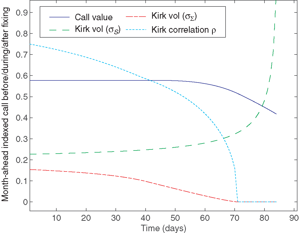
As an example, we first study the behavior of month-ahead indexed call options, which will serve as decomposition products for a swing. Figure 2 shows the call value and the Kirk parameters of a daily month-ahead indexed option written on the thirteenth of the respective month. The valuation period begins long before the fixing starts, then runs through the fixing period and ends thirteen days after the last fixing. The graph illustrates how a month-ahead indexed option approaches the Black-76-type option as time runs to the end of the fixing period. In this example, during the last thirteen days of the option’s lifetime, it coincides with a plain vanilla option with a fixed strike.

4.2 Decomposition of a swing contract

For simplicity, we consider an at-the-money fixed-strike swing option on gas in the Dutch Title Transfer Facility (TTF) hub with delivery period October 2016 to September 2017. We suppose it to be subject to one annual constraint (${\text{ACQ}}_{\min }=90,{\text{ACQ}}_{\max }=120$) and 365 identical daily constraints (${\text{DCQ}}_{\min }=0,{\text{DCQ}}_{\max }=1$), ie, we have

	${\mathrm{\Pi }}_1$	$=\{10/01/16,10/02/16,\mathrm{\dots },09/30/17\}$
	${\mathrm{\Pi }}_2$	$=\{10/01/16\},$
	${\mathrm{\Pi }}_3$	$=\{10/02/16\},$
		$\mathrm{⋮}$
	${\mathrm{\Pi }}_{366}$	$=\{09/30/17\}.$

Moreover, the swing contract is decomposed into monthly products (monthly futures, options and time-spread options), ie, $I_i^{\mathrm{F}}=I_i^{\mathrm{C}}=I_i^{\mathrm{L}}=I_i^{\mathrm{S}}$, $i=1,\mathrm{\dots },12$, are assumed to be the monthly delivery periods. These products are valued as of September 1, 2016 using a monthly forward curve and a flat monthly volatility surface of 21%. To account for the spot dynamics, we use a seasonal cash volatility: ${\sigma }_{\text{cash},\text{summer}}=100$% and ${\sigma }_{\text{cash},\text{winter}}=120$%.

Table 1: Decomposition of an at-the-money fixed-strike swing. [Decomposition of a 90–120 at-the-money fixed-strike swing contract for GY2016/2017 and corresponding option and future values. We assumed a flat forward volatility surface of 21%, a seasonal cash volatility of ${\sigma }_{\text{cash},\text{summer}}=\text{100}$% and ${\sigma }_{\text{cash},\text{winter}}=\text{120}$% as well as an artificial monthly forward curve with a typical yearly pattern.]

(a) Forward positions
		Volume	Value
	Delivery	(MWh)	(€/MWh)
	Jan 2017	30	0.29
	Feb 2017	01	0.19
	Mar 2017	31	$-$0.01
	Apr 2017	28	$-$0.71
(b) Call positions
		Volume	Value
	Delivery	(MWh)	(€/MWh)
	Sep 2017	30	0.98
(c) Time spread call positions
		Volume	Value
Long leg	Short leg	(MWh)	(€/MWh)
Nov 2016	Jan 2016	30	0.37
Dec 2016	Feb 2016	01	0.61
Dec 2016	Mar 2016	30	0.74
Jan 2017	Mar 2016	01	0.86
Feb 2017	Apr 2016	28	1.30

Figure 3: Illustration of a monthly swing decomposition. Illustration of the value-optimizing choice of a swing decomposition into monthly products. For example, the value of 30 (solid black curve) in January refers to a January future delivering 30 MWh in total over the entire month. The green long-dashed line showing, for example, 31 in December indicates that all time-spread options together swap a maximum of 31 MWh in total from other months into December. Correspondingly, the blue short-dashed line showing, for example, $-$31 in March means all time-spread options swap a maximum of 31 MWh in total out of March into the other months.

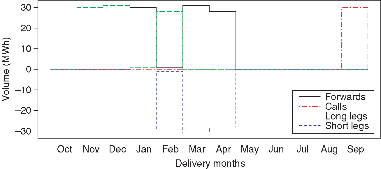
The fair values of the decomposition products and the value-optimizing choice of those products can be found in Table 1 as well as Figure 3. In this case, the swing is replicated by four futures, one call option and five time-spread calls. As can easily be seen, this decomposition satisfies the swing restrictions: ${\text{ACQ}}_{\min }=90$ is logged in by futures. Those futures cover the short legs of the five time-spread options, which retain the flexibility to swap to other delivery months that are not yet blocked by another product. Finally, the optionality ${\text{ACQ}}_{\max }-{\text{ACQ}}_{\min }=30$ is exploited using a call option.

4.3 Comparison with standard LSMC approach

In this section, we compare the NPV results obtained by our pricing approach to a standard LSMC approach, which has been calibrated to market quotes. The LSMC approach is based on a normal mean-reverting market model that has proven decent consistency with sensitivities to the forward curve level as well as the forward volatility level. As an example, we study a month-ahead indexed swing contract for a gas year with the “as-of” day one month before delivery.

Note that the presented valuation approach and the LSMC valuation algorithm are fundamentally different. We propose a static decomposition of a swing in contrast to the dynamic spot optimization approach of LSMC. While we consider LSMC as a reference figure, it does not serve as a benchmark. In fact, we expect severe discrepancies, which are disclosed and analyzed below.

Toward this end, we will consider various flexibility classes, ie, various values of ${\text{ACQ}}_{\max }$ and ${\text{ACQ}}_{\min }$. This means our calculations comprise products that are rather dissimilar, namely, a pure strip of options (${\text{ACQ}}_{\max }=365$ and ${\text{ACQ}}_{\min }=0$), a pure forward position (${\text{ACQ}}_{\max }=365$ and ${\text{ACQ}}_{\min }=365$), a time spread without optionality (${\text{ACQ}}_{\max }={\text{ACQ}}_{\min }$) and any combination of these. It has turned out to be a nontrivial problem to find a valuation methodology that provides market reflective swing values for the entire flexibility matrix. In practice, we therefore narrow this task to the most liquidly traded areas, while for illustrative purposes we will provide the entire flexibility matrix here.

Figure 4: Results compared with LSMC. Results of our swing valuation approach (center), LSMC swing values applied to a mean-reversion process ($\kappa =\text{4.0}$) (left) and deviations of the two (right) in €/MWh for several swing flexibilities with a month-ahead indexed strike. The columns show different values of ${\text{ACQ}}_{\text{max}}$ and the rows show MinTake ratios ($={\text{ACQ}}_{\text{min}}/{\text{ACQ}}_{\text{max}}$). We assumed a flat forward curve of 18.5€/MWh, a flat annual forward volatility term structure of 21.0% and a flat cash volatility of 120%. We used valuation date September 1, 2017, delivery period October 2017 to September 2018.

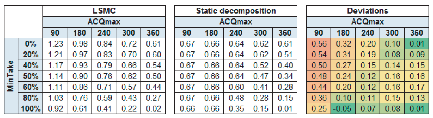
Figure 4 shows the partly diverging behavior of the two valuation approaches. For large values of ${\text{ACQ}}_{\max }(\ge 180)$ and low values of ${\text{ACQ}}_{\min }$ we observe a decent consistency. For small ${\text{ACQ}}_{\max }$ values, however, our decomposition approach does not exploit as much value as LSMC. The reasons for this are manifold, so we would like to stress two particularly important aspects.

First, compared with our decomposition approach, the LSMC shows a better capability to exploit the value of a Bermudan-type option. Consider the edge case, where ${\text{ACQ}}_{\max }=1$, ${\text{ACQ}}_{\min }=0$ and the delivery period is one year. In other words, the holder of the swing has the right to exercise one option at any time within the delivery year. In this case, our approach values the swing by choosing the single most valuable daily European-type option of the year while neglecting any additional value due to the swing’s inherent Bermudan exercise rights. The LSMC approach is able to exploit more of this value, particularly if applied to a strongly mean-reverting underlying process. Thus, in this example, it provides a swing value significantly above the most valuable European-type option. This can be understood by decreasing the mean-reversion rate $\kappa$ of the underlying process while keeping its terminal variance constant and again applying the LSMC. Due to the lower mean reversion, we assign less value to a Bermudan-type optionality and obtain a better consistency between the two approaches.

Second, as outlined in Section 3.2.1, we approximate the time-spread option values by only taking into account the cash variances. We neglect any value that is driven by the forward dynamics of the underlying spread legs. Thus, we slightly undervalue the time-spread optionality, which leads to a small value lag, particularly for swings with high ${\text{ACQ}}_{\max }$ and ${\text{ACQ}}_{\min }$ constraints, ie, swings that contain a significant portion of time-spread value.

In an ad hoc approach, this can be compensated for by increasing the cash variances in the time-spread valuation, while keeping it unchanged for outright options. This is essentially equivalent to a separate calibration of cash variances for outright options and time-spread options. These results suggest that the market-implied cash variances for outright options and time-spread options are in fact different. This is a very important observation that traders should be aware of when hedging a swing with Greeks obtained by this valuation approach.

Figure 5: Dynamic Delta hedge of month-ahead indexed swing. Evolution of swing value, dynamic Delta hedge and dispatch strategy of 0–182 month-ahead indexed swing contract. With a cash volatility of (a) 100% and (b) 40%, we obtain initial values of €99 and €69, respectively (constant forward volatility 16.7%). Delivery period: July 1, 2015 to December 31, 2015 (182 days). The plots show the differences between values at trade inception and current values.

Figure 6: Moneyness and Delta of month-ahead indexed swing. (a) Moneyness and (b) monthly Delta of 0–182 month-ahead indexed swing contract (parameterization as above). The monthly Delta exposure is almost zero prior to the fixing period. During the fixing period, the monthly Delta increases linearly due to the underlying month-ahead indexed product successively approaching a fixed-strike product. Eventually, during delivery, the Delta exposure decreases to zero, since we are only considering the contract for its remaining delivery days.

4.4 Backtesting the pricing strategy

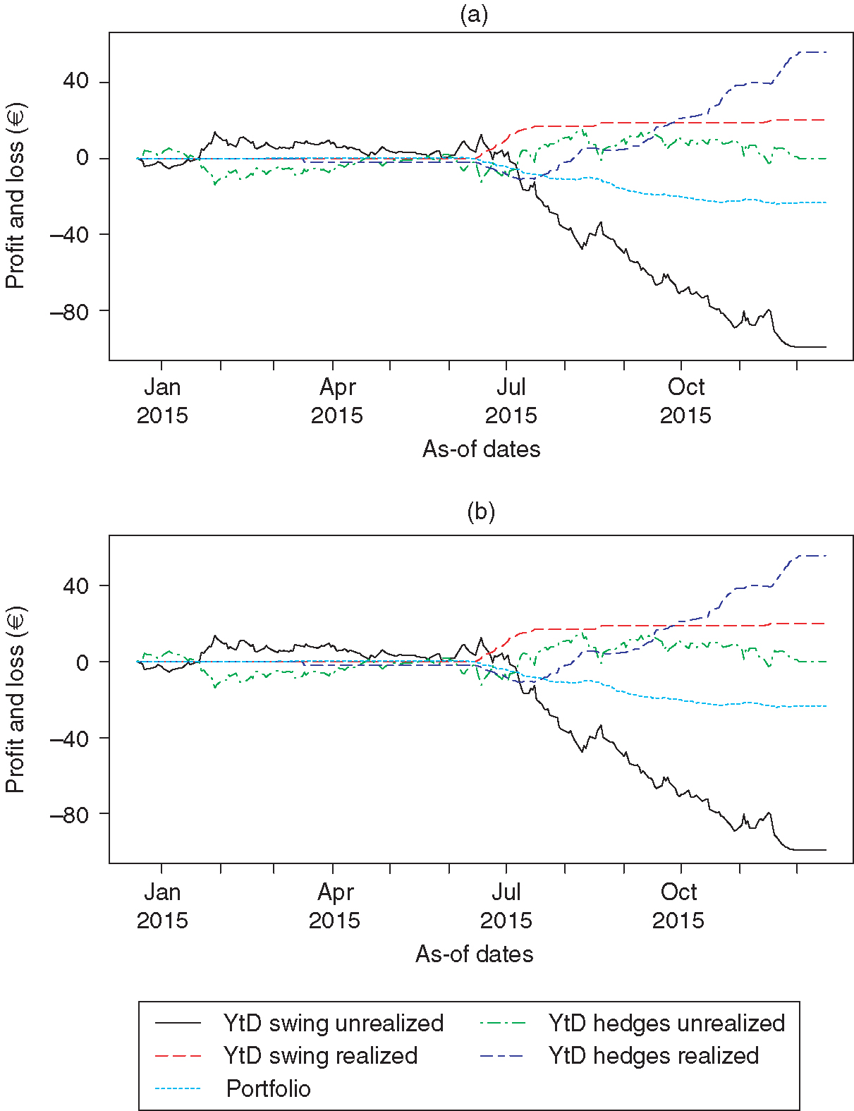
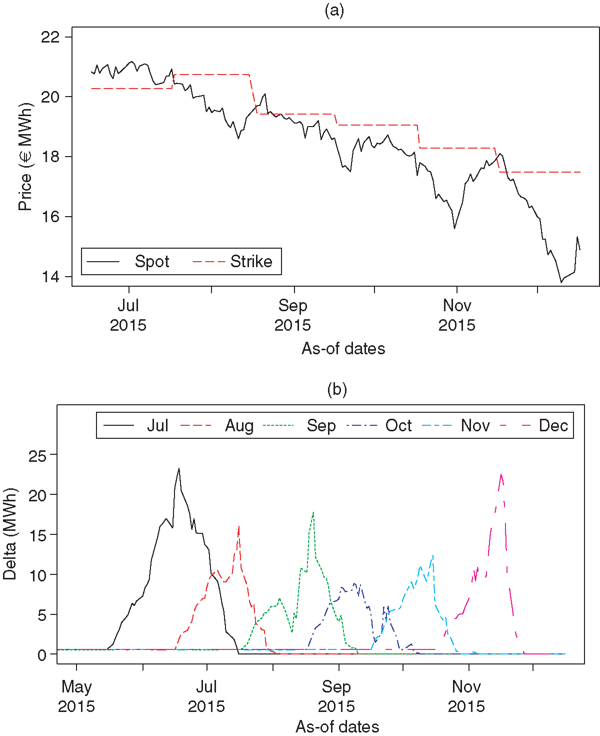
For backtesting purposes, we evaluated a month-ahead indexed swing using the methodology described above. The contract’s delivery period is July 1, 2015 to December 31, 2015 (182 days). Between January 2, 2015 and end of delivery, the contract is reevaluated and Delta-hedged on a daily basis using historical forward curves as well as a constant historical forward volatility and a constant cash volatility. Transaction costs are neglected in this analysis. As hedge products, we allow the next thirty-one days, five months and two quarters.

The results with a commonly used cash volatility of 100% are illustrated in Figure 5(a). Long before delivery, the Delta replication of the month-ahead indexed swing performs very well. Losses in the indexed swing mark-to-model value are fully compensated by profits in the Delta portfolio and vice versa. In any case, due to very low Deltas, the profit and loss (PnL) changes in this period are of minor importance. Only as late as one month before delivery is the first Delta significantly increasing, as the first monthly index is gradually fixed (see Figure 6). With an increasing Delta, we can also observe larger PnL fluctuations of the replication portfolio. The first month’s Delta reaches its peak at the first day of delivery and then decreases, since the remaining swing product successively rolls over the first month. Meanwhile, the second month’s Delta gains in value and peaks one month later, and so on.

Moreover, when the delivery period is reached, the swing is exercised as per the dispatch strategy, ie, in this case whenever the payoff is positive. Since this is the case almost exclusively in the first month of delivery (see Figure 5(a)), the swing product itself is only profitable in this first delivery month. In the subsequent months, the swing does not get back into the money, which leads to a quick value decrease that is not tracked by the Delta. We thus can observe a rather poor hedge performance in these months. However, as we know from the pricing methodology, the analytic month-ahead indexed swing value is highly sensitive to the cash volatility. Consequently, the same applies to the Deltas and the hedge performance. In this respect, the underperformance of the hedge suggests the swing-implied cash volatility is larger than the actual cash volatility. Indeed, the historically averaged cash volatility in this period has only been around 40%. Adjusting the cash volatility accordingly leads to a better performing replication strategy (see Figure 5(b)). Apart from the remaining averaging error, other sources of inaccuracies are rather manageable: for reasonable choices of forward prices and volatilities, the moment-matching approximation errors in the outright and time-spread option valuation algorithms are negligibly small, particularly close to expiry. Neglecting the forward dynamics in the valuation of indexed time-spread options is also a very accurate approximation over a very large range of forward values, which means this is effectively irrelevant for the Deltas as well.

5 Conclusion

In this paper, we provided an efficient alternative to the common swing option pricing methods by decomposing the contract into tradable products. We extended the existing Keppo method by additionally exploiting a swing option’s Bermudan properties, ie, we added time-spread optionality. We found approximative solutions to apply our methodology to both fixed strike and indexed swing options. For illustration purposes, we showed a step-by-step application of our technique to a commonly traded month-ahead indexed swing option. Moreover, we calculated analytical expressions for the Greeks and showed, using historical data, their ability to closely replicate the swing option’s price fluctuations. In a comparison with a standard LSMC valuation approach, we saw that the consistency of the results strongly depends on the flexibility class of the swing option. We suggested an ad hoc way to further improve this consistency over all flexibility classes; namely, to separately calibrate the cash volatilities for different option types. Of particular use for practitioners, our methodology constitutes a transparent and computationally less involved alternative to the most commonly used Monte Carlo pricing methods.

Declaration of interest

The authors report no conflicts of interest. The authors alone are responsible for the content and writing of the paper.

References

• Barrera-Esteve, C., Bergeret, F., Dossal, C., Gobet, E., Meziou, A., Munos, R., and Reboul-Salze, D. (2006). Numerical methods for the ppricing of swing options: a stochastic control approach. Methodology and Computing in Applied Probability 8(4), 517–540 (https://doi.org/10.1007/s11009-006-0427-8).
• Brigo, D., and Mercurio, F. (2006). Interest Rate Models: Theory and Practice. Springer (https://doi.org/10.1007/978-3-540-34604-3).
• Broadie, M., and Glasserman, P. (2004). A stochastic mesh method for pricing high-dimensional American options. The Journal of Computational Finance 7(4), 35–72 (https://doi.org/10.21314/JCF.2004.117).
• Carmona, R., and Durrleman, V. (2003). Pricing and hedging spread options. SIAM Review 45(4), 627–685 (https://doi.org/10.1137/s0036144503424798).
• Carmona, R., and Touzi, N. (2008). Optimal multiples stopping and valuation of swing options. Mathematical Finance 18(2), 239–268 (https://doi.org/10.1111/j.1467-9965.2007.00331.x).
• Dahlgren, M. (2005). A continuous time model to price commodity-based swing options. Review of Derivatives Research 8(1), 27–47 (https://doi.org/10.1007/s11147-005-1006-9).
• Jaillet, P., Ronn, E. I., and Tompaidis, S. (2004). Valuation of commodity-based swing options. Management Science 50(7), 909–921 (https://doi.org/10.1287/mnsc.1040.0240).
• Keppo, J. (2004). Pricing of electricity swing options. Journal of Derivatives 11(3), 26–43 (https://doi.org/10.3905/jod.2004.391033).
• Kirk, E. (1995). Correlation in the energy markets. In Managing Energy Price Risk, Kaminsk, V. (ed), pp. 71–78. Risk Books, London.
• Lari-Lavassani, A., Simchi, M., and Ware, A. (2001). A discrete valuation of swing options. Canadian Applied Mathematics Quarterly 9(1), 35–73.
• Li, M., Zhou, J., and Deng, S.-J. (2010). Multi-asset spread option pricing and hedging. Quantitative Finance 10(3), 305–324 (https://doi.org/10.1080/14697680802626323).
• Longstaff, F., and Schwartz, E. (2001). Valuing American options by simulation: a simple least-squares approach. Review of Financial Studies 14(1), 113–147 (https://doi.org/10.1093/rfs/14.1.113).
• Margrabe, W. (1978). The value of an option to exchange one asset for another. Journal of Finance 33(1), 177–186 (https://doi.org/10.2307/2326358).
• Pellegrino, T., and Sabino, P. (2014a). On the use of the moment-matching technique for pricing and hedging multi-asset spread options. Energy Economics 45, 172–185 (https://doi.org/10.1016/j.eneco.2014.06.014).
• Pellegrino, T., and Sabino, P. (2014b). Pricing and hedging multiasset spread options using a three-dimensional Fourier cosine series expansion method. The Journal of Energy Markets 7(2), 71–92 (https://doi.org/10.21314/JEM.2014.117).
• Venkatramanan, A., and Alexander, C. (2011). Closed form approximations for spread options. Applied Mathematical Finance 18(5), 447–472 (https://doi.org/10.1080/1350486x.2011.567120).
• Wilhelm, M., and Winter, C. (2008). Finite element valuation of swing options. The Journal of Computational Finance 11(3), 107–132 (https://doi.org/10.21314/JCF.2008.191).

Download PDF

• Keywords
• Decomposition
• Energy markets
• Swing options
• Original research