Journal of Risk Model Validation
ISSN:
1753-9587 (online)
Editor-in-chief: Steve Satchell
Credit portfolio stress testing using transition matrixes
Radu Neagu, Gabriel Lipsa, Jing Wu, Jake Lee, Stephane Karm and John Jordan
Need to know
- We present a method for stress testing credit portfolios using transition probability matrices.
- We benchmark our method against two competing methods and backtest out-of-sample.
- Out-of-sample period chosen to be the 2008 financial crisis (to resemble a stress period).
- All methods are conservative out-of-sample, overestimating default rates; ours proves closest.
Abstract
In this paper, we propose a new methodology for modeling credit transition probability matrixes (TPMs) using macroeconomic factors. We use two indicators, which we call bias and inertia, to summarize the properties of a given TPM. The dependence of a TPM on the economic cycle is achieved by linking the bias and inertia to macro- economic variables using regression modeling techniques. A TPM reconstruction algorithm (for given values of the bias and inertia parameters) is used, together with exogenous stressed future values for the macroeconomic factors, to produce stressed projections of portfolio default rates (DRs). We compare, out-of-sample and using a data set from Moody’s Credit Risk Calculator, results using this new methodology with results using two other competing methodologies. The out-of-sample period is chosen to coincide with the 2008 financial crisis, to resemble a stressed period; this is an appropriate and innovative backtesting exercise, given that the methods discussed here are stress-testing methods. We find that, overall, the method we propose outperforms the other two competing methods. For the in-sample performance, our method outperforms the other two during the 2001 dot-com bubble; however, it lags during the expansion period leading up to the 2008 financial crisis.
Introduction
1 Introduction
Understanding, evaluating and managing credit risk is a priority for any financial institution, GE Capital Corporation (GECC) included. Until June 2016, GECC qualified as a nonbank systemically important financial institution (SIFI) and was therefore subject to comprehensive supervision by the Board of Governors of the Federal Reserve System (Fed). While GECC has never taken part in the Comprehensive Capital Analysis and Review (CCAR) and Dodd-Frank Act (DFA) stress tests,11 1 See https://bit.ly/2Ihr1wR for details on CCAR and DFA. or their European equivalent,22 2 See http://www.eba.europa.eu/risk-analysis-and-data/eu-wide-stress-testing. it was required to provide results from stressing its credit portfolio under various macroeconomic stress scenarios. More precisely, GECC’s Enterprise Stress Testing (EST) efforts were motivated by the need for a forward-looking evaluation of the impact of stressful economic and financial market conditions on the firm. These stressful conditions are based on internally developed scenarios; the models provide estimates of the potential future losses associated with the GECC portfolio (at an enterprise-wide as well as a business-unit level) under the various stressed economic scenarios. The results are used for capital and risk management purposes. The work presented in this paper stems from these requirements, the growing importance of having stress-testing frameworks/capabilities and the necessity of linking credit portfolio losses to macroeconomic factors.
This paper details one approach to addressing these challenges. Stress-testing models are notoriously difficult to backtest as they are designed to predict events that have a low probability of occurring and are therefore missing from most historical training data sets. Given the growing importance of stress-testing models, we feel that employing adequate model-testing techniques is essential. We propose a training/validation split for our analysis data set that enables us to perform this backtesting. GECC has historically assumed that credit rating transitions follow a Markovian process modeled vis-à-vis transition probability matrixes (TPMs; see, for example, Keenan et al 2008; Long et al 2011; Zhang et al 2010). TPMs are matrixes that contain estimates of the probabilities of obligors transitioning from their current credit rating (represented by rows in the matrix) to any other rating including default (represented by columns in the matrix) over a predetermined time period (one year is common practice). (For more details on TPMs, see, for example, Inamura (2006) and the references therein.) It has been noted that credit transitions may follow non-Markovian processes (Lando and Skødeberg 2002). Others have published methods for testing this property (Bangia et al 2002; Arvanitis et al 1999), and still others have shown that non-Markovian behavior can be approximated by using Markov mixture models (Frydman and Schuermann 2008) or semi-Markovian models (Koopman et al 2008). Our tests for momentum and duration on our own internal portfolio data yielded mixed results, leading us to conclude that there was enough support for the Markovian assumption not to be violated. Consequently, because of the methods and results presented in this paper, we do not view it as a limiting assumption.
The use of TPMs for credit portfolio stress testing is widespread in the industry, and, due to the growing importance of stress testing, the number of relevant studies is quite large. We provide here a few examples, not meant as an exhaustive list. Bangia et al (2002) present a framework for stress testing the loss distribution of credit portfolios, where credit migration matrixes provide the specific linkages between underlying macroeconomic conditions and expected changes in the credit quality of obligors. Similarly, Jafry and Schuermann (2004) present a method based on the singular values of transition matrixes to estimate economic credit risk capital during periods of economic stress. Miu and Ozdemir (2009) present a methodology for estimating stressed PDs and migration rates conditioned on macroeconomic variables under stress scenarios. The authors use this methodology for stress testing at the overall portfolio level as well as for specific industries. More recent examples include Sobehart (2018), Perilioglu et al (2018), Yang (2017) and Skoglund (2017). Also, there have been many researchers who have noted the dependence of TPMs on the business cycle (Fons 1991; Belkin et al 1998; Bangia et al 2002; Nickell et al 2000; Koopman and Lucas 2005; Carling et al 2007; Sobehart 2008; Belotti and Crook 2009).
Two primary techniques have been used for computing TPMs: cohort and continuous (for details on these methods, please see, for example, Inamura (2006) and Lando and Skødeberg (2002)). Although each technique yields different TPMs (Jafry and Schuermann 2004; Lando and Skødeberg 2002), GECC has chosen to compute TPMs using the cohort approach, after it was determined that the continuous approach resulted in higher default rate (DR) prediction errors over multiple periods (Long et al 2011). In this paper, we propose a methodology to link TPMs to macroeconomic factors by using two matrix summary features called bias and inertia. Bias represents the ratio between upgrades and downgrades, while inertia represents the likelihood that an obligor will stay in the same rating category during the chosen time period (a type of mobility metric). Data from Moody’s is used for our analysis: quarterly rating transitions are pulled from Moody’s Credit Risk Calculator (CRC), with 1994 Q3–2007 Q3 used as the training set and 2007 Q4–2010 Q3 used as the validation set. We chose the validation set specifically to cover the 2008 financial crisis (stressed environment), so we use actual values for the macroeconomic factors during that episode. We also have, out-of-sample, the actual realized DRs, which we use to assess the performance of our method and of the alternatives considered. We test our proposed methodology, as well as two competing alternatives available in the literature, by predicting (out-of-sample) DRs during the 2008 financial crisis. We do this for three reasons. First, we want to benchmark our method against other available alternatives. Second, we are interested in gauging and backtesting the performance of these methods out-of-sample (we also briefly discuss in-sample performance). Third, we chose the out-of-sample period to be the episode of the 2008 financial crisis. Since the models discussed in this paper are meant to produce estimates for stressed business cycles, and given the magnitude of the 2008 financial crisis, this choice of validation set aligns well with our intended use for the models. Also, since losses are ultimately produced by defaults and not migration to nondefault classes, we focus our numerical results discussion on the performance of stressed default rates rather than stressed TPMs. We show that the method presented in this paper predicts the DRs well and, overall, outperforms our (best) implementations of the other two methods (which we present here in brief).
This paper is organized as follows. In Section 2, we give more details about the data set used. Section 3 presents details about the bias and inertia (BI) methodology as well as out-of-sample results. In Section 4, we discuss three competing methods and present out-of-sample results for two of them. In Section 5, we compare results from our BI methodology with those from the two alternative methods. Section 6 summarizes our conclusions and discusses future research directions.
2 The data
As discussed in the introduction, we use rating transition data from Moody’s CRC ranging from 1994 Q3 to 2010 Q3, where 1994 Q3 to 2007 Q3 is used for model training and 2007 Q4 to 2010 Q3 is used for out-of-sample backtesting.
The CRC database is built directly on Moody’s Default & Recovery Database, which has rich historical data going back several decades. As such, rating transition data is available from as early as 1970. At the same time, for major macroeconomic variables such as gross domestic product (GDP) and unemployment, long historical time series data is available. However, spread variables such as high-yield spread (HYS), Aaa spread and others that closely relate to credit events were only available to us starting from 1994 Q3. Consequently, for the analysis presented in this paper, we chose a sample starting from 1994 Q3 onward. We restrict ourselves to data from the United States for all industries. Table 1 shows a summary of this data by quarter.
| Total | DR | Total | DR | ||||
|---|---|---|---|---|---|---|---|
| Date | obl. | Defaults | (%) | Date | obl. | Defaults | (%) |
| 1994 Q3 | 1807 | 6 | 0.33 | 2002 Q4 | 2486 | 15 | 0.60 |
| 1994 Q4 | 1824 | 2 | 0.11 | 2003 Q1 | 2447 | 16 | 0.65 |
| 1995 Q1 | 1842 | 2 | 0.11 | 2003 Q2 | 2415 | 18 | 0.75 |
| 1995 Q2 | 1858 | 8 | 0.43 | 2003 Q3 | 2411 | 17 | 0.71 |
| 1995 Q3 | 1894 | 7 | 0.37 | 2003 Q4 | 2392 | 10 | 0.42 |
| 1995 Q4 | 1934 | 9 | 0.47 | 2004 Q1 | 2418 | 7 | 0.29 |
| 1996 Q1 | 1975 | 4 | 0.20 | 2004 Q2 | 2453 | 8 | 0.33 |
| 1996 Q2 | 2022 | 4 | 0.20 | 2004 Q3 | 2477 | 5 | 0.20 |
| 1996 Q3 | 2068 | 1 | 0.05 | 2004 Q4 | 2463 | 10 | 0.41 |
| 1996 Q4 | 2114 | 7 | 0.33 | 2005 Q1 | 2499 | 5 | 0.20 |
| 1997 Q1 | 2191 | 4 | 0.18 | 2005 Q2 | 2520 | 4 | 0.16 |
| 1997 Q2 | 2242 | 6 | 0.27 | 2005 Q3 | 2524 | 11 | 0.44 |
| 1997 Q3 | 2324 | 5 | 0.22 | 2005 Q4 | 2532 | 9 | 0.36 |
| 1997 Q4 | 2396 | 6 | 0.25 | 2006 Q1 | 2534 | 4 | 0.16 |
| 1998 Q1 | 2481 | 9 | 0.36 | 2006 Q2 | 2555 | 4 | 0.16 |
| 1998 Q2 | 2597 | 9 | 0.35 | 2006 Q3 | 2574 | 6 | 0.23 |
| 1998 Q3 | 2715 | 5 | 0.18 | 2006 Q4 | 2569 | 5 | 0.19 |
| 1998 Q4 | 2750 | 17 | 0.62 | 2007 Q1 | 2587 | 3 | 0.12 |
| 1999 Q1 | 2768 | 14 | 0.51 | 2007 Q2 | 2595 | 5 | 0.19 |
| 1999 Q2 | 2810 | 26 | 0.93 | 2007 Q3 | 2606 | 3 | 0.12 |
| 1999 Q3 | 2824 | 15 | 0.53 | 2007 Q4 | 2608 | 2 | 0.08 |
| 1999 Q4 | 2837 | 20 | 0.70 | 2008 Q1 | 2601 | 13 | 0.50 |
| 2000 Q1 | 2824 | 22 | 0.78 | 2008 Q2 | 2571 | 16 | 0.62 |
| 2000 Q2 | 2808 | 33 | 1.18 | 2008 Q3 | 2555 | 18 | 0.70 |
| 2000 Q3 | 2754 | 16 | 0.58 | 2008 Q4 | 2522 | 28 | 1.11 |
| 2000 Q4 | 2748 | 33 | 1.20 | 2009 Q1 | 2467 | 60 | 2.43 |
| 2001 Q1 | 2710 | 32 | 1.18 | 2009 Q2 | 2387 | 70 | 2.93 |
| 2001 Q2 | 2684 | 37 | 1.38 | 2009 Q3 | 2315 | 40 | 1.73 |
| 2001 Q3 | 2658 | 35 | 1.32 | 2009 Q4 | 2271 | 19 | 0.84 |
| 2001 Q4 | 2626 | 37 | 1.41 | 2010 Q1 | 2286 | 12 | 0.52 |
| 2002 Q1 | 2546 | 30 | 1.18 | 2010 Q2 | 2304 | 7 | 0.30 |
| 2002 Q2 | 2521 | 24 | 0.95 | 2010 Q3 | 2349 | 8 | 0.34 |
| 2002 Q3 | 2516 | 21 | 0.83 |
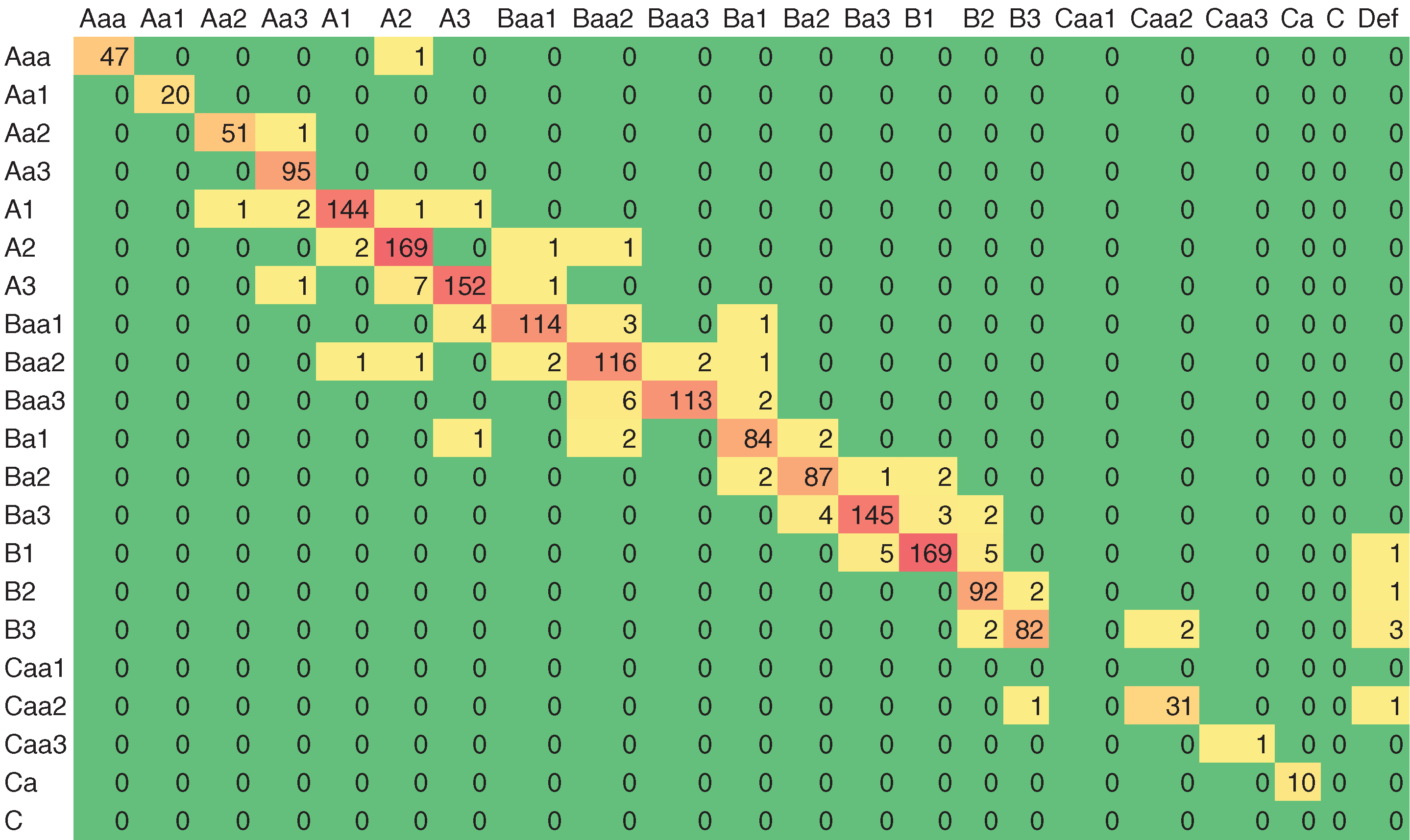
As mentioned in the introduction, we use the cohort method over quarterly time periods to compute the empirical TPMs. The instances that become withdrawn during the calculation time period (quarter) are excluded. By excluding withdrawn ratings, the default rate calculation is conservative, since Moody’s tracks defaults for a minimum of one year after an issuer withdraws its rating. If the issuer first withdraws and then defaults within the quarter, the issuer will be shown as defaulted and so be counted; those that do not default will not be counted. Figure 1 shows an example of such a quarterly empirical TPM computed for the 1994 Q3 cohort (we show counts rather than percentages; to convert them, we would divide each cell by the row totals).

The empirical TPM is concentrated on the diagonal and, overall, default counts are zero for investment grade. Consequently, we decided to combine the obligors in the investment grade categories as well as those in the speculative grades Caa2 to C. Since the transition period for computing the TPM is a quarter, there are very few observed defaults in the low risk grades, and most migration probabilities are zero. This results in very sparse data in the low-risk area of the granular matrixes. Hanson and Schuermann (2006) give a good analysis of the differentiation between probabilities of default associated with notch- and grade-level classes in the investment and speculative grade areas. They conclude (in a discussion at the top of p. 2292 of that paper): “Thus even at the whole grade level, dividing the investment grade into four distinct groups seems optimistic from the vantage point of PD estimation.” They also state that: “In the speculative grade range … one is much more clearly able to distinguish default probability ranges at the notch level.” We took these results to heart and decided to collapse grades in the fashion we did. In the case of a high credit quality portfolio, this method of collapsing grades would not be ideal; further analysis of alternative ways to prepare the data would be needed. Since the focus of this paper is on modeling methodologies, we list this study as an area for future work. For the analysis presented in this paper, we use these coarse rating categories (nine credit ratings plus default). The resulting empirical TPM for the 1994 Q3 cohort is presented in Figure 2.

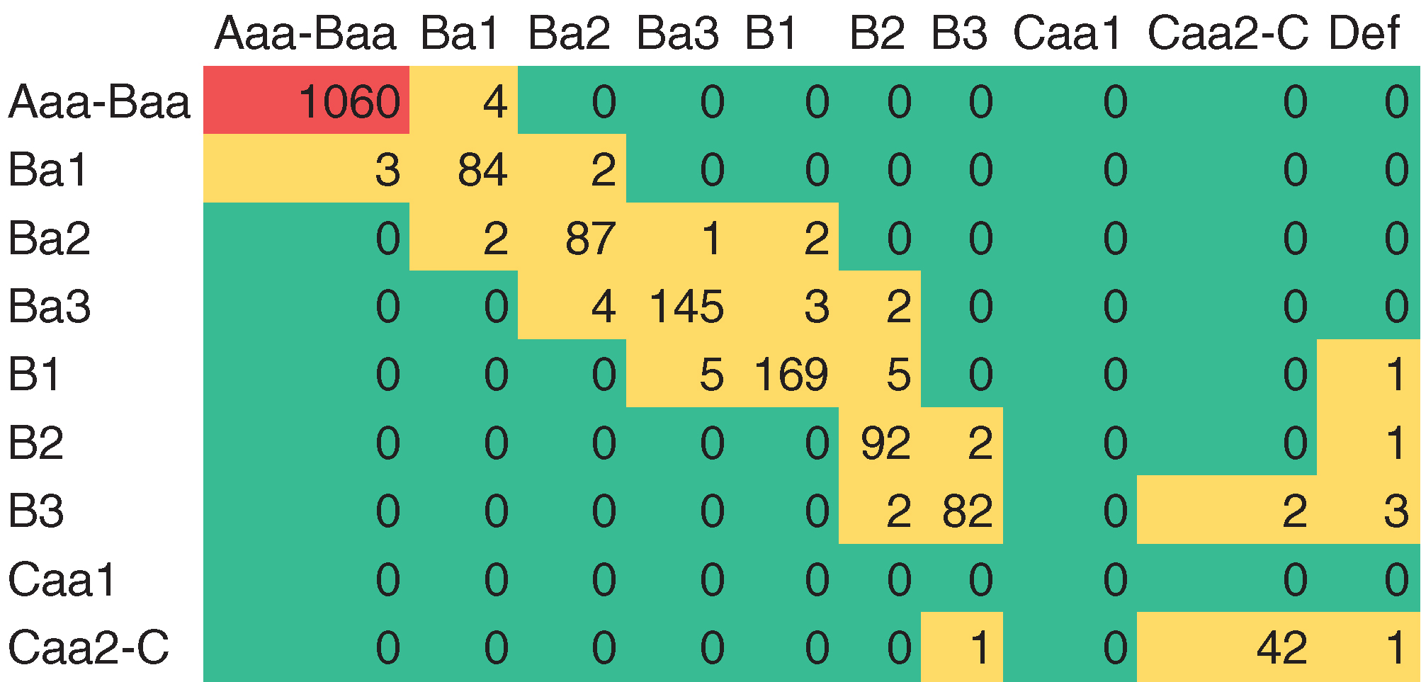
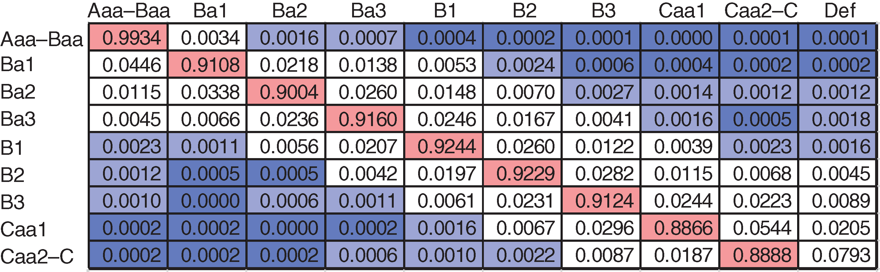
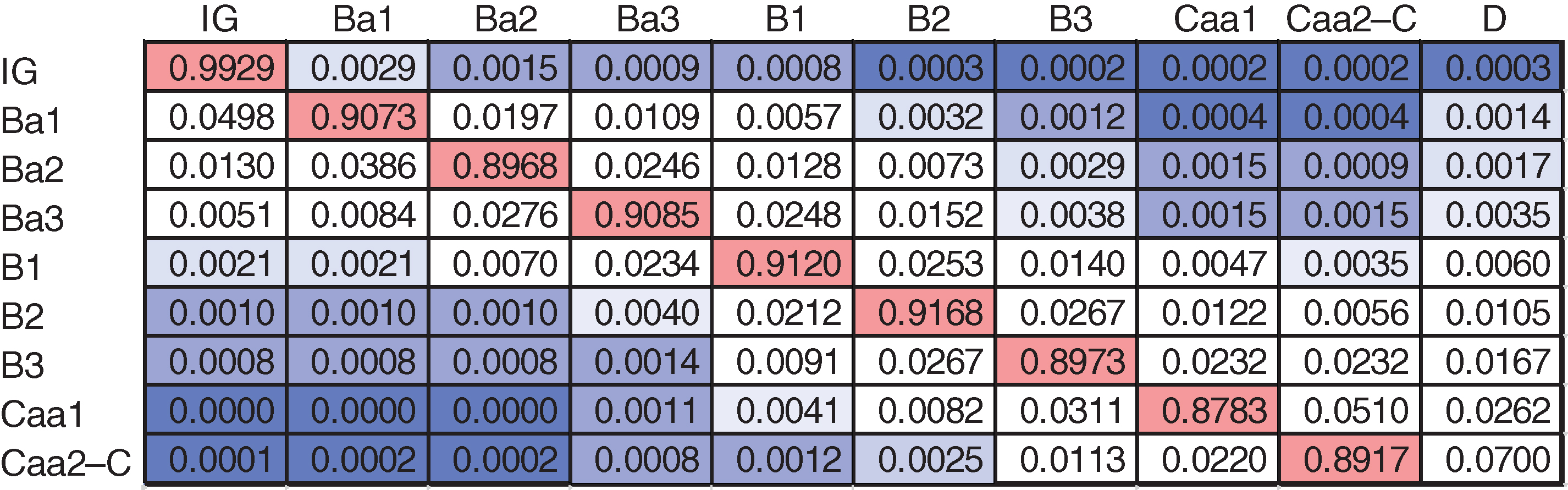
Figure 3 shows the average one-quarter empirical TPM computed across the training data set. The default rate for the Aaa–Baa category is 1 basis point (bp): the magnitude of this number further supports our decision to collapse classes into this category. In addition, the decision to keep Caa1 separate from the rest of the C classes was driven by the difference seen in the empirical default rate: 0.0205 versus 0.0793.

Finally, because of the low default rate in the Aaa–Baa category, the large count associated with this category does not impact our results in a material way. A more detailed discussion on this subject is given in Section 3.4.
We also make use of data on macroeconomic factors over the period 1994 Q3–2010 Q3 (our GE internal data management team pulled this information from publicly available sources). We use three different transformations on the data: quarterly annualized growth (QA), quarterly absolute difference (Delta) and spread in reference to five-year interest rates (R5Y). In addition, two derived variables are used as candidates in the variable selection process–yield curve (the difference between a ten-year rate and a three-month Treasury bill interest rate) and TED spread (the difference between a three-month London Interbank Offered Rate (Libor) and a three-month Treasury bill interest rate). Table 2 shows all available variables and their transformation methods.
3 Bias and inertia (BI) methodology
In this section, we present details about our methodology as well as the numerical results obtained when applying this method to the analysis data set. All methods presented are applied to the same ratings and macroeconomic data.
3.1 Methodology flowchart
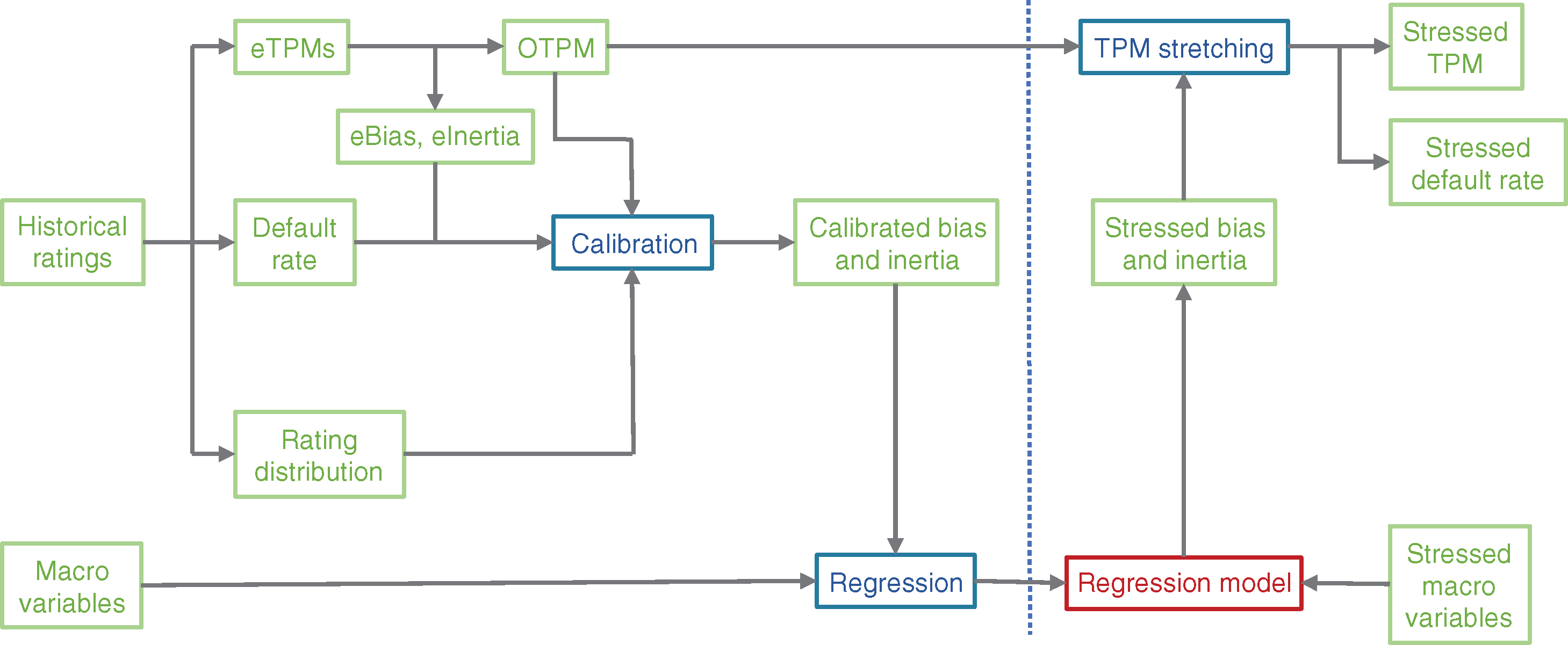
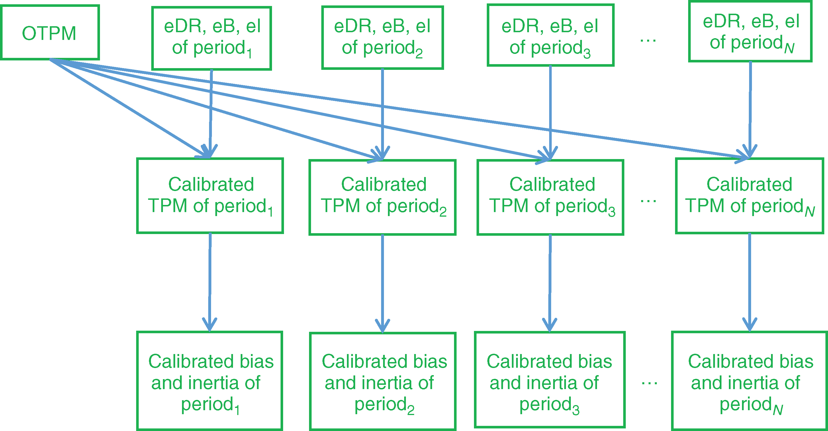
The main idea behind the method in this paper is to use a (small) set of metrics that can characterize key information contained in the TPM; in this way, we avoid using the entire matrix (which could increase the complexity/dimensionality significantly). Additional details about this methodology can be found in Keenan et al (2008). Figure 4 outlines the steps/flow of our model.
eTPM stands for empirical TPM, eBias and eInertia stand for empirical bias and inertia, and OTPM stands for the optimized TPM. These items will be discussed in more detail later in this section. As the diagram in Figure 4 shows, we use historical data to compute the empirical TPMs, DRs, rating distributions, eBias and eInertia as well as the OTPM. Using eBias and eInertia, the OTPM, the DR and the rating distribution, we calibrate the model to compute the calibrated bias and inertia. We then use historical values for the macroeconomic variables together with the calibrated bias and inertia to build regression functions linking the two. Plugging stressed values for the macroeconomic variables into the regression functions outputs the stressed bias and inertia. By using these, together with the OTPM, we compute the stressed TPM (through an operation we call stretching) and consequently the stressed DR.
3.2 Bias and inertia
| Calc. | ||
|---|---|---|
| Code | method | Description |
| GDP | QA | NIPA: gross domestic product (USD billions (2009), SAAR) |
| U | Delta | Household survey: unemployment rate (%, SA) |
| STR | Delta | Interest rates: federal funds rate (% PA, NSA) |
| LTR | Delta | Interest rates: ten-year constant maturity securities |
| (% PA, NSA) | ||
| HPIPO | QA | FHFA purchase-only home price index |
| (index 1991 Q1 100, SA) | ||
| CPI | QA | CPI: urban consumer – all items |
| (index 1982–84 100, SA) | ||
| YDisp | QA | Income: disposable personal (USD billions (2009), SAAR) |
| WTI | QA | Petroleum crude oil spot price: West Texas Intermediate |
| (USD per barrel, NSA) | ||
| NG | QA | NYMEX natural gas futures prices: contract 1 |
| (USD per MMBtu) | ||
| HYS | Delta | High-yield bonds: option adjusted spread (%, NSA) |
| Aaa | R5Y | Moody’s intermediate-term bond yield average: |
| corporate – rated Aaa (%, NSA) | ||
| Aa | R5Y | Moody’s intermediate-term bond yield average: |
| corporate – rated Aa (%, NSA) | ||
| A | R5Y | Moody’s intermediate-term bond yield average: |
| corporate – rated A (%, NSA) | ||
| Baa | R5Y | Moody’s intermediate-term bond yield average: |
| corporate – rated Baa (%, NSA) | ||
| RPrim | Delta | Interest rates: bank prime rate (% PA, NSA) |
| R5Y | Delta | Interest rates: five-year constant maturity securities |
| (% PA, NSA) | ||
| R30Y | Delta | Interest rates: thirty-year constant maturity securities |
| (% PA, NSA) | ||
| R1M | Delta | Libor rates: one-month USD deposits (% PA, NSA) |
| R3M | Delta | Libor rates: three-month USD deposits (% PA, NSA) |
| R6M | Delta | Libor rates: six-month USD deposits (% PA, NSA) |
| R1Y | Delta | Libor rates: one-year USD deposits (% PA, NSA) |
| YInd | QA | Industrial production: total (index 2007 100, SA) |
| VIX | Delta | S&P 500 volatility (thirty-day MAVG, NSA) |
| SP5 | QA | S&P stock price index: 500 composite |
| (index 1941–43 10; monthly average, NSA) | ||
| HPI | QA | FHFA all transactions home price index |
| (index 1980 Q1 100, NSA) | ||
| YWage | QA | Income: wages and salaries – total (USD billions, SAAR) |
| HPICS | QA | Case–Shiller monthly home price index: |
| 20-metro composite (index 2000 Q1 100, SA) | ||
| RMort | Delta | Terms conventional mortgages: all loans – fixed |
| effective rate (%, NSA) | ||
| RT3M | Delta | Interest rates: three-month Treasury bills – secondary |
| market (% PA, NSA) | ||
| R7Y | Delta | Interest rates: seven-year constant maturity securities |
| (% PA, NSA) | ||
| HPIC | QA | Flow of funds: commercial real estate price index |
| (index, SA) | ||
| YCV | LTR-RT3M | Yield curve |
| TED | R3M-RT3M | TED spread |

Details about the calculation of bias and inertia can be found in Keenan et al (2008). We briefly review these definitions here. Assume we have the following transition matrix:
where is the number of ratings (including default, symbolized by the last row/column). We define inertia as
| (3.1) |
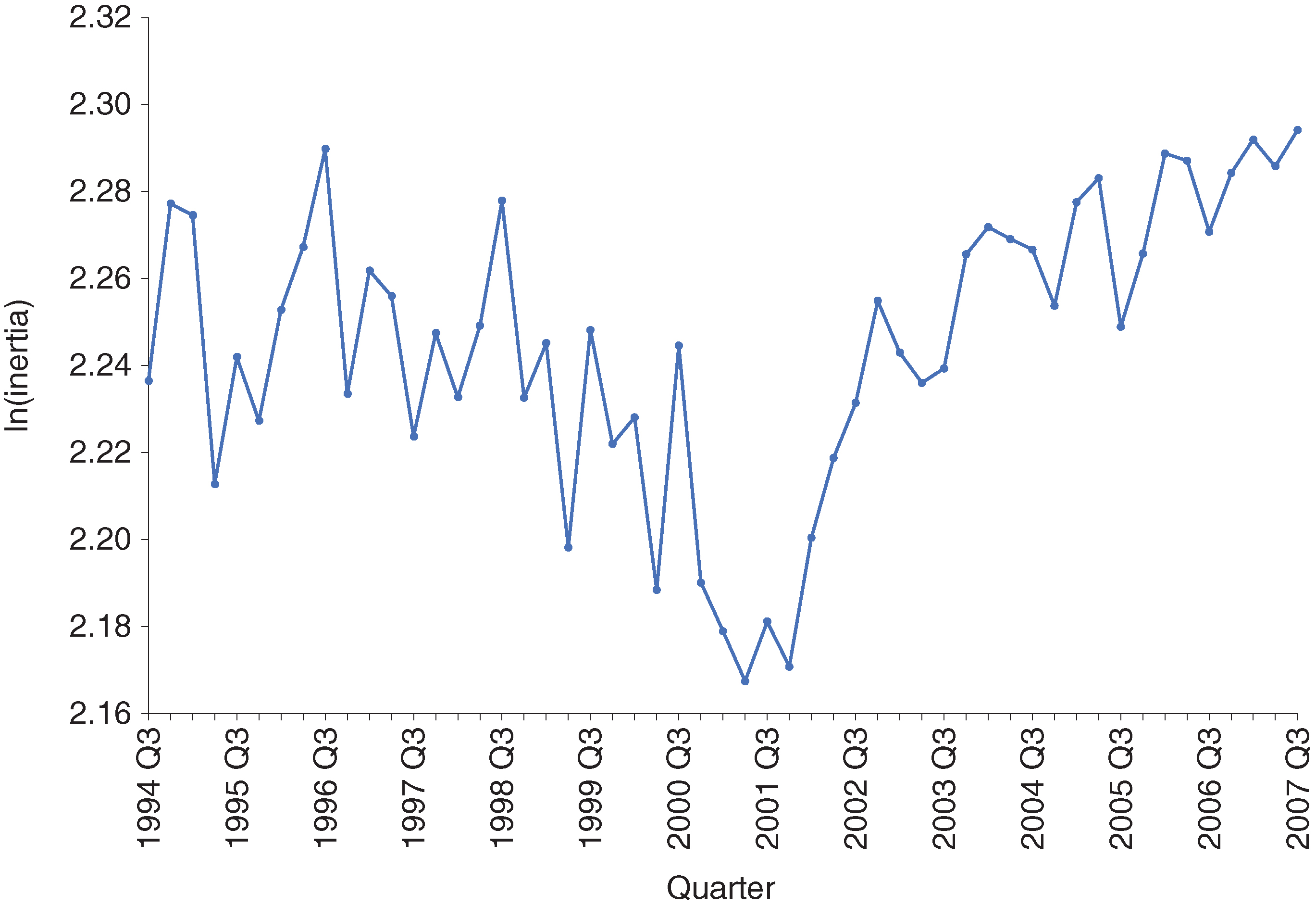
Inertia can be interpreted as the likelihood that an obligor stays in the same rating category over a fixed time period (a quarter, in our case). A declining inertia value indicates higher rating volatility (ie, a higher probability of migrating out of a rating category), while a high value indicates lower rating volatility (ie, a lower probability of migrating out of a rating category). Figure 5 shows the for the analysis data set.

The second feature is the bias, defined as
| (3.2) |
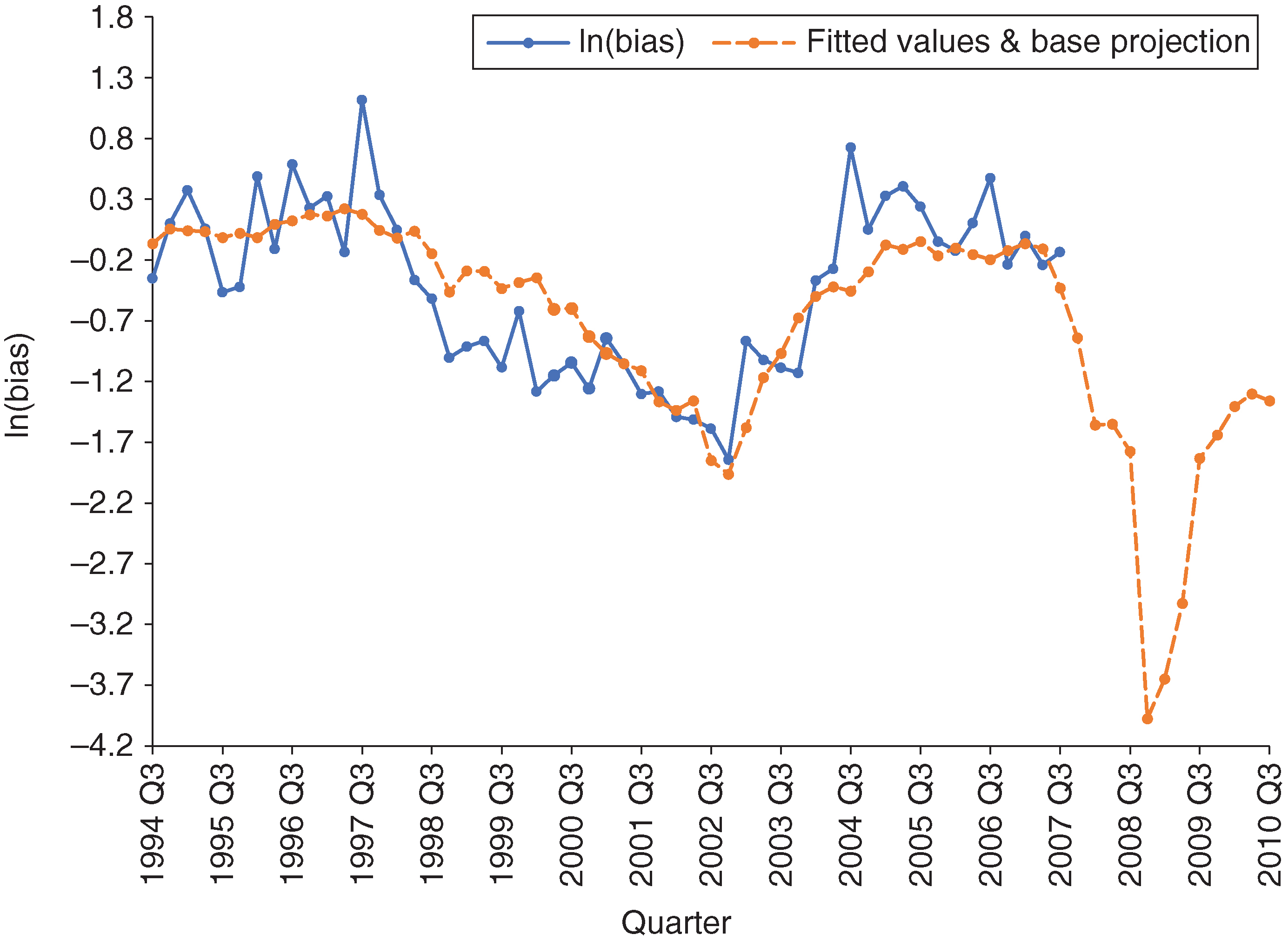
Note that the numerator is the summation of the probabilities below the main diagonal (corresponding to upgrades), while the denominator is the summation of the probabilities above the main diagonal (corresponding to downgrades). Hence, bias is a ratio between upgrade and downgrade mass for a TPM. If the bias is greater than , there are more upgrades than downgrades, while a value below represents more downgrades than upgrades. Figure 6 shows the for the analysis data set.

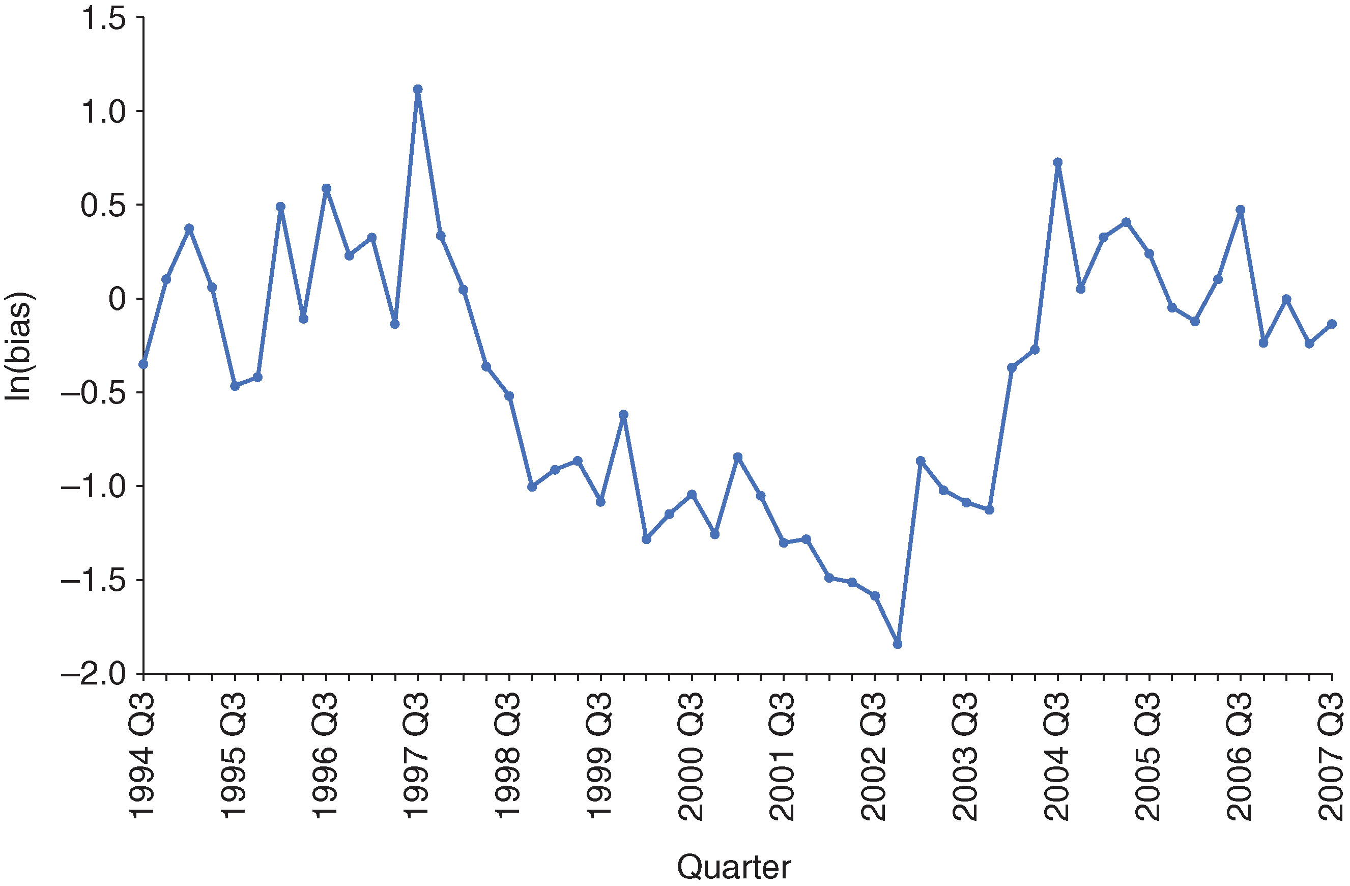
The correlation between the bias and inertia series is 0.42. This low value indicates the fact that the bias and inertia effectively capture different dynamic features of the TPM. Others have also used upgrade-to-downgrade ratios and/or trace to summarize TPMs and to track rating transition trends (see Sobehart and Keenan 2004; Sobehart 2008; Jafry and Schuermann 2003, 2004; Okashima and Fridson 2000; Trück 2004). In choosing the bias and inertia, we were motivated by two main requirements: capturing the mobility and upgrade/downgrade ratio of the TPM; and increasing simplicity/reducing dimensionality. We are aware, as is always the case when simplifying an approach/method, that we miss some of the aspects contained in the full TPM. We list a few ideas for future research in the conclusions section.
3.3 Optimized TPM
Details about the calculation of the OTPM can be found in Long et al (2011), Keenan et al (2008) and Zhang et al (2010). We briefly review this concept here.
The OTPM is computed as the solution of the following optimization problem:
| (3.3) |
where is the empirical multiperiod TPM for the period from to , are weights given to each period and are weight matrixes that control how much weight is placed on each of the entries of the TPM ( spans all quarters in the data). The norm is the element-wise Euclidean norm, although other distance functions could also be used, and the multiplication between the and OTPM matrixes is element-wise. The intuition around the OTPM is as follows. The stress-testing exercise requires tracking the evolution of a portfolio over multiple periods of time (quarters), and therefore it is only natural to model sequential migrations of obligors (including the migration into the default state). We accomplish this by using TPM multiplication as an approximation to multiperiod migration. We are therefore looking for a matrix (the OTPM) that, when multiplied with itself, provides optimal approximations to empirical multiperiod transition matrixes. This OTPM is computed in a way that minimizes the difference between the series of OTPMs raised to increasing powers and the corresponding multiperiod empirical TPMs over time windows of up to twelve quarters across the entire data set.
The weights are introduced so that different time periods can get “customized” emphasis in the optimization. We generally assign higher weights to shorter horizons (1 Q, 2 Q, etc), decreasing the weight as the time horizon increases (to match the fact that our confidence decreases as we increase the time horizon). For this paper, we use a linearly decreasing series where and . All entries are equal to for the matrixes used, so we did not employ any differentiation.
Finally, properties of the OTPM are discussed in detail in Zhang et al (2010). In particular, the method used to solve the optimization in (3.3) is a self-adaptive differential evolution algorithm with a representation schema that satisfies certain constraints imposed on the OTPM (such as monotonicity off the main diagonal). This method was chosen especially because of concerns about finding global optimums rather than ending in local ones, which was the case with other methods (namely, the nonlinear programming methods or basic evolutionary algorithms) discussed in Zhang et al (2010). The quality of the ultimate solution (rather than other metrics, such as computation speed) was emphasized and drove the implementation of the final optimization algorithm.
The resulting OTPM for the training data set is given in Figure 7.

3.4 Calibration
The calibration process generates the calibrated bias and inertia, computed from a calibrated TPM denoted . Parameters , for the transformation are computed by solving an optimization problem in which the empirical DR, bias and inertia are approximated. Figure 8 depicts the calibration process.

To formalize the calibration process, we define several functions. The first function is one that computes the default rate:
| (3.4) |
where is a matrix and is a weights vector such that , . The DR function outputs the weighted sum of the DRs of each row. We use weights that are proportional to the count of obligors in each row.
We define to be the bias of (given by (3.2)) and to be the inertia of (given by (3.1)). We also define a transformation of a given TPM as a function of two parameters and , , in steps (a) and (b), as follows.
- Step (a):
-
apply an adjustment to the diagonal elements based on the value of , then adjust the off-diagonal elements such that (i) after adjustment each row sums to ; (ii) the ratio of sum of upgrades to sum of downgrades for each row is preserved; (iii) the ratio between any two upgrade (or downgrade) cells in each row is preserved:
- Step (b):
-
to the output of step (a) (ie, the matrix ), apply an adjustment to the ratio of the sum of upgrade cells to the sum of downgrade cells based on the value of :
Intuitively, if, for example, (the opposite holds if ), we want to (i) leave the main diagonal unchanged (to preserve the inertia); (ii) lower the total upgrade probability of the matrix (lower triangle) by the amount (); (iii) ensure each row sums to ; and (iv) for each row, adjust the remaining (downgrade) cells by the same (row-specific) quantity. As a result, when the bias of the resulting matrix will be lower. Under these requirements/constraints, it can easily be shown that
With the definitions laid out above, we have
where is the upgrade mass of row in matrix and is the downgrade mass of row in matrix ().
This transformation gives us the ability to change a TPM in such a way that the result is another TPM that achieves (in an approximate way) predefined bias and inertia values. This process of transforming a given matrix to achieve predefined bias and inertia values is also referred to as “stretching”, explained below. The transformation plays a key role in the calibration as well as the stretching steps.
With these concepts defined, and for each period of time (quarter), we compute a set of parameters and that satisfies the following minimization problem:
| (3.5) |
where TPM is the empirical transition matrix for that period. For the function, the weights are calculated using the empirical TPMs for each period and are applied to both the TPM and the matrix (first term in (3.5)). This is the only place where the large counts for the Aaa–Baa category come into play: the weight given to this category will be significantly higher than the other weights. However, because of the very low default rates for the Aaa–Baa category in the OTPM as well as the empirical and average TPMs, the impact of the magnitude of the weight placed on this category is negligible (as a percentage of the value of the function). If anything, it biases the results to find better matches for the Aaa–Baa category, possibly at the expense of the other classes. But, again, this impact is negligible.
The , , constants are defined beforehand and act as weights for the three terms in the objective function. Since they are constants defined outside the minimization in (3.5), we could factor out constant and interpret the values of and as weights to control the relative importance to place on bias and inertia relative to the default rate. For proprietary reasons, we do not disclose the values of , and that we used; their values were selected based on a set of simulation studies.
In the sequence of steps outlined in Figure 4, one of the most challenging is the reconstruction of the stressed TPM given target (stressed) values for the bias and inertia. We do this reconstruction using the process of “stretching”, which will be discussed in detail in the next section. In that process, we start with a base TPM (we chose the OTPM), apply the transformation to obtain “customized” bias and inertia values, and then optimize , to best match the given target values for the bias and inertia. Since, in the end, our choice for the projected stressed TPM is the resulting , we want to go back over the range of our in-sample historical data, construct these matrixes (for each quarter ) to best match the empirical data (therefore, the objective function in (3.5)), and use the bias and inertia of these matrixes (rather than the bias and inertia of the empirical TPMs) to build the linkage models to the macroeconomic factors. This is the calibration process, and the resulting bias and inertia are the calibrated bias and calibrated inertia. It provides consistency between the way we construct the future stressed TPMs and the process we use to estimate the parameters needed for those constructions. For each quarter, (3.5) will solve for a pair of parameters (, ), which, in turn, define the matrix . This defines the calibrated bias, , and the calibrated inertia, , which are the quantities linked to the macroeconomic factors through the regression equations (to be discussed next).
3.5 Regression models and stretching
For the regression models, we use a list of macroeconomic factors (as described in the data section) to obtain a transfer function that explains the calibrated bias and inertia. As response variables, the log transforms of the calibrated bias and inertia are used. To select the macroeconomic factors that have the strongest predictive power for credit migration, we first conduct a correlation analysis between them (including their lags) and the log transforms of the calibrated bias and inertia. Table 3 summarizes the correlation analysis (the figures in bold indicate statistically significant sample correlation).
| Macro. no lag | Macro. lag (1) | Macro. lag (2) | Macro. lag (3) | Macro. lag (4) | ||||||
| GDP | 30 | 18 | 34 | 38 | 2 | 2 | 7 | 14 | 5 | 17 |
| U | 23 | 19 | 14 | 39 | 13 | 34 | 10 | 27 | 13 | 24 |
| SP5 | 2 | 25 | 31 | 21 | 40 | 38 | 13 | 27 | 11 | 4 |
| Baa | 30 | 36 | 40 | 48 | 5 | 37 | 11 | 14 | 21 | 18 |
| HYS | 18 | 41 | 34 | 8 | 23 | 26 | 13 | 14 | 22 | 1 |
| TED | 1 | 11 | 31 | 18 | 28 | 36 | 17 | 23 | 6 | 18 |
Based on the correlation analysis, we boiled down our selection of macroeconomic factors and their lags to a smaller subset that is significantly correlated with both and . These variables are SP5, Baa, GDP, U and HYS. We performed three different modeling techniques for variable selection: time series regression, principal component regression and stepwise regression. Due to its simplicity, ease of interpretation and comparable performance, we decided to select the final models using stepwise regression. We concluded that the model for bias contains only Baa (no lag) and the model for inertia contains only U (no lag). Figures 9 and 10 show in-sample fits as well as projections from these two models.


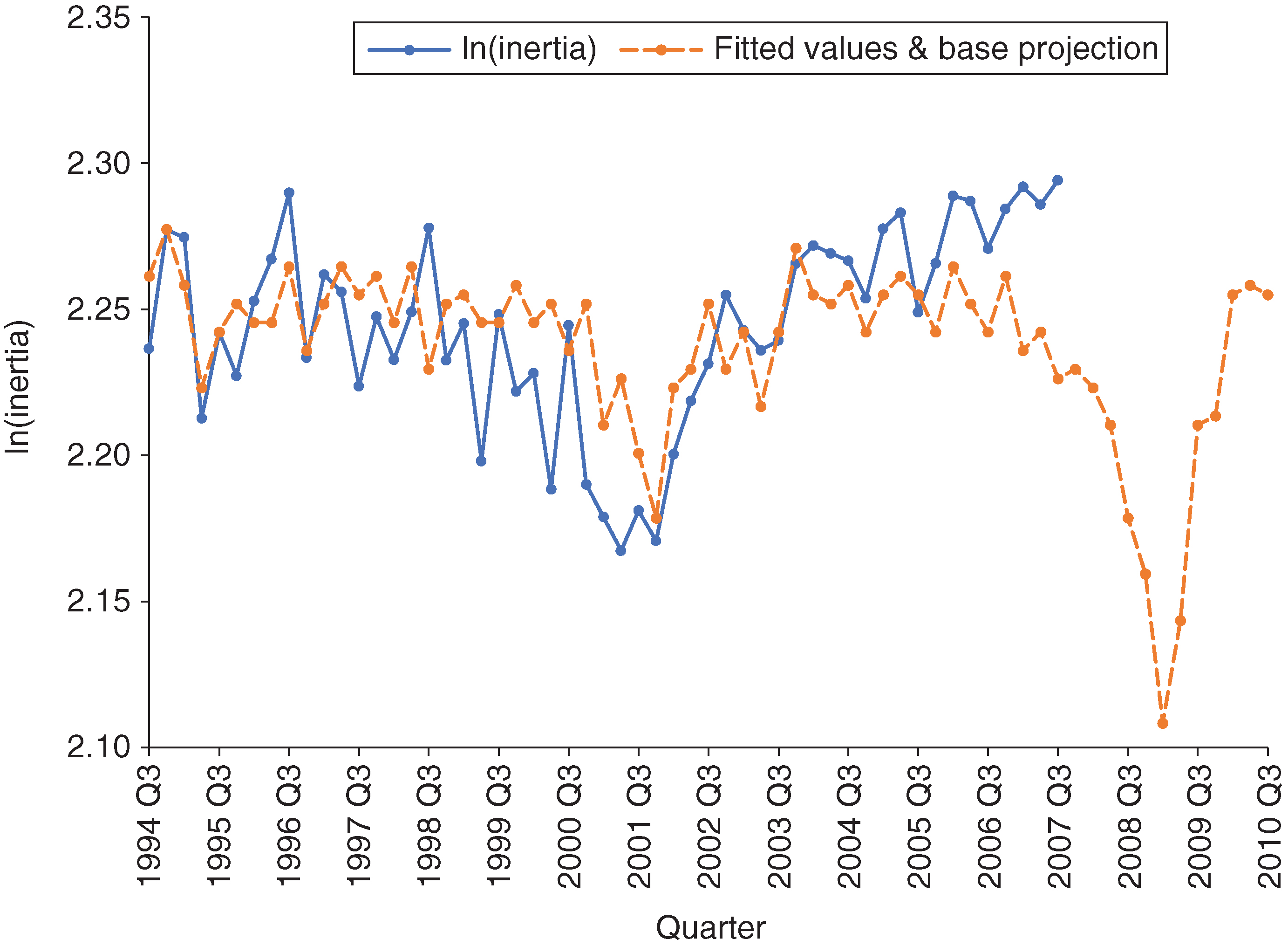
For the inertia model, we observe a deviation in the model fit at the end of the in-sample period. The reason for this gap is an increase in the unemployment rate in that period, which drags down the model-fitted value. We expect this will impact the forecasting performance. We will come back to this point later in this section.
Using the regression models and the stressed macroeconomic data (in our case, the actual values during the 2008 financial crisis), we derive the stressed bias and inertia, which represent the targets we want to come closest to when constructing the stressed TPMs. Our stressed TPM is given by ; we just need to estimate the values for the and parameters that result in this matrix having the closest bias and inertia to the target values, a process we call “stretching”. Since, as discussed in the previous section, the bias and inertia formulas for , as functions of the parameters and , are not as simple as one would like (and therefore analytical solutions are quite difficult), we solved this by employing the objective function and minimization problem in (3.6) below:
| (3.6) |
The resulting stretched TPM is given by , with the optimal pair from (3.6). The stressed TPM is that obtained when using the stressed bias and inertia as target values. In our experience of applying this method to the data in this paper as well as to a number of internal GE portfolios, we did not run into convergence issues (for the minimization problems in (3.5) and (3.6)). We are using the “fmincon” MATLAB solver.
3.6 Numerical results
In this section, we discuss the results from applying our proposed method to the analysis data. As mentioned earlier, we use the 2008 financial crisis as an out-of-sample validation set for our model. Since losses are ultimately produced by defaults and not migration to nondefault classes, we focus on the performance of stressed default rates rather than stressed TPMs. We therefore compare the projected DR to the observed DR as a means of gauging model performance.
Figure 11 shows the fit of our model to the actual DR, where the out-of-sample period is identified by the rectangular box.

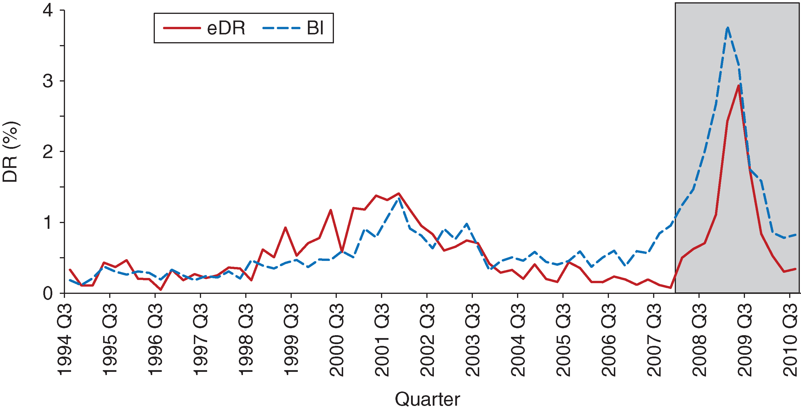
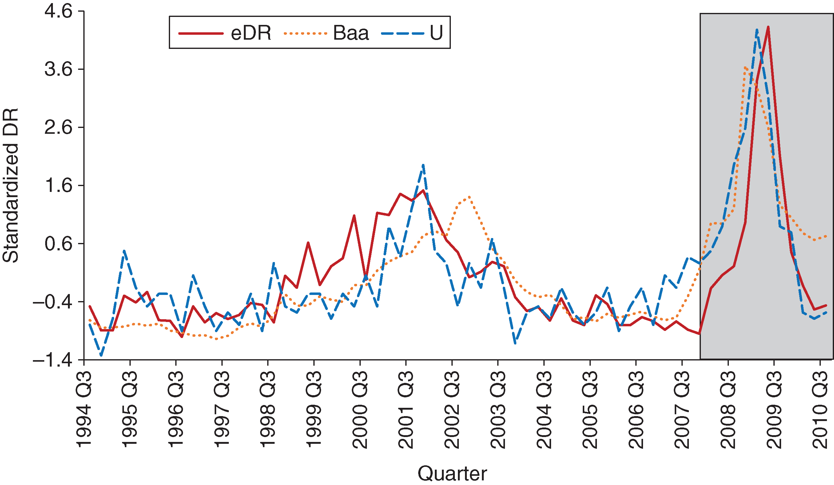
The in-sample performance is good, capturing the level and trend quite accurately. Where the model’s fit is not as strong is during the period leading up to the end of the training sample. There we overpredict the DR, a trend that carries into the out-of-sample period. We can track our overprediction of the DR to the deviation of the macroeconomic factors used in the regression model from the actual DR. Figure 12 shows the (standardized) macroeconomic factors used in the bias and inertia regression models together with the actual DR. Probably the gap between our out-of-sample projected DR and the actual DR could be narrowed by choosing other factors in the regression models. However, our attempts at doing so were unsuccessful and the results presented herein are the most performant.
Out-of-sample, the maximum difference between the projected DR and the actual DR is 0.84%, the mean absolute error is 0.75% and the sum of squared errors is 0.09% (the latter two metrics are discussed in more detail in, for example, Trück (2008)).

4 Alternate methodologies
4.1 Moody’s method
Moody’s method (Licari et al 2013) analyzes the TPM by looking at all upgrade or downgrade notches of the same order together (ie, all one-notch transitions together, all two-notch transitions together, etc). Analyzing the one-notch transitions together is being justified by the fact that there is interdependence between the one-notch upgrades and one-notch downgrades. The two-notch or higher transitions have a different structure. Moody’s proposal is to use a regime-switching model combined with a regression model for notch transitions. Forecasting is accomplished by performing a principal component analysis of the one-notch transitions (downgrade and upgrade probabilities); for the results presented here, we used the first three principal components. The macroeconomic variables used in the regression are GDP growth, U and Baa; we add GDP because it is found to be significant for the model. We did not use a formal method for choosing these variables; they were selected after several trial-and-error iterations. Our intention was also to use similar variables to those in the BI methodology. Those interested in more details are encouraged to read Licari et al (2013).
4.2 Moody’s methodology results
In this section, we conduct the same out-of-sample comparison between the DR estimates obtained using the method in Licari et al (2013) and the actual DR.
Similar to the analysis in Section 3, we use the 2008 financial crisis as our validation set. The two-notch transitions are modeled using the same approach as for the one-notch transition. The in-sample and out-of-sample results are presented in Figure 13.

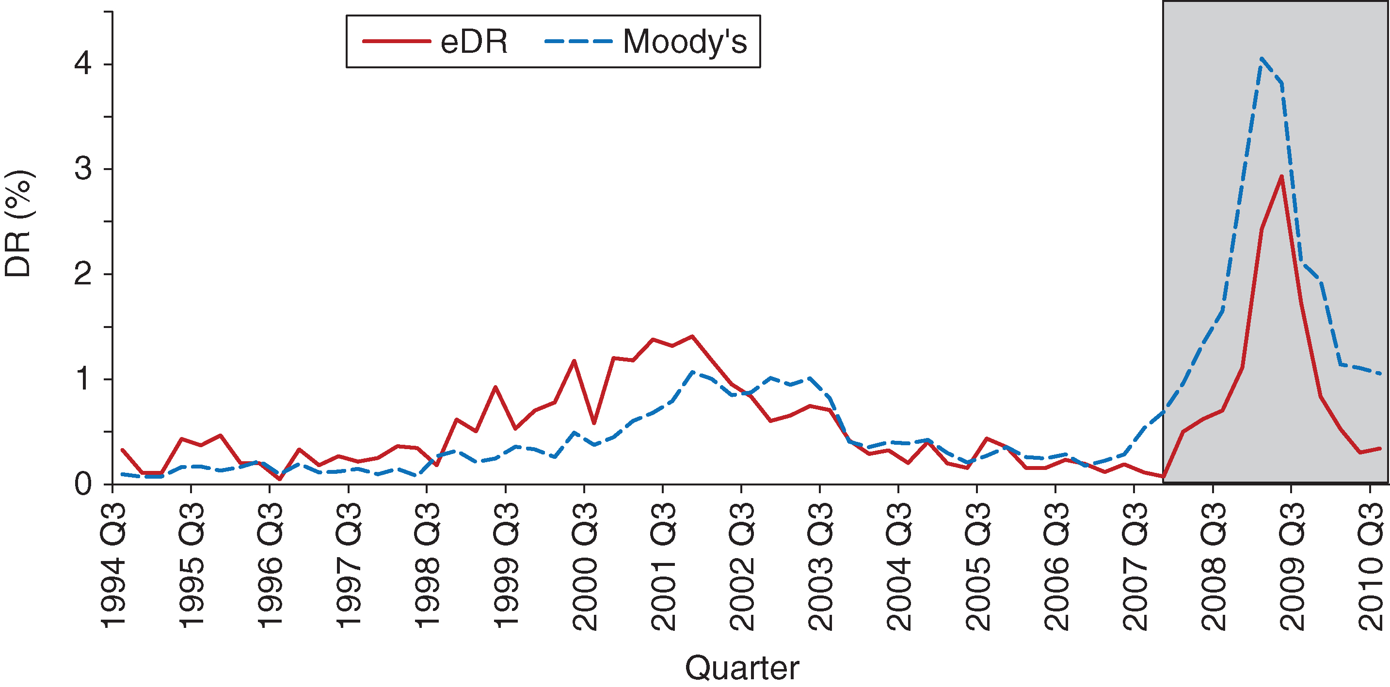
While we see a divergence between actual DR and model DR estimates around the 2001 dot-com bubble, the fit is better, when compared with our method, in the period leading up to the 2008 financial crisis. However, out-of-sample, our method marginally outperforms Moody’s model: the maximum difference between the projected DR and the actual DR is 1.1%, the mean absolute error is 0.89% and the sum of squared errors is 0.11%. The timing of the peak is accurate for both models, with Moody’s DR estimates being less conservative leading up to the peak. After the peak, our estimates drop faster and to lower levels, which is more in tune with the observed DR.
4.3 Bank of Japan methodology (Otani et al 2009)
This model was proposed by (Wei 2003) and explains the fluctuations in the transition probabilities for all rating categories. Due to space constraints, we focus on the results; readers interested in more details are encouraged to read the referenced papers. Note that in Otani et al (2009) the macroeconomic factors used are GDP and unemployment, but other factors can be added. Also note that the methodology used is proposed for borrowers in five categories: normal, needs attention, special attention, in danger of bankruptcy, de facto bankrupt or bankrupt. This method was not designed for credit ratings on a scale similar to Moody’s (or Standard & Poor’s). Since these are the scales we use in this paper, we are unsure of the effect this assumption has on the final results.
4.4 Bank of Japan methodology results
In this section, we conduct the same out-of-sample comparison between the DR estimates obtained using the method in Otani et al (2009) and the actual DR. Again, like the analyses in the previous sections, we use the 2008 financial crisis as our validation set. The selection of the macroeconomic factors for the regression model is done using a greedy algorithm, where we start with the collection of macroeconomic variables presented in Table 2. The final macroeconomic indicators chosen are Baa, YCV and R30Y.
The in-sample and out-of-sample results are presented in Figure 14.

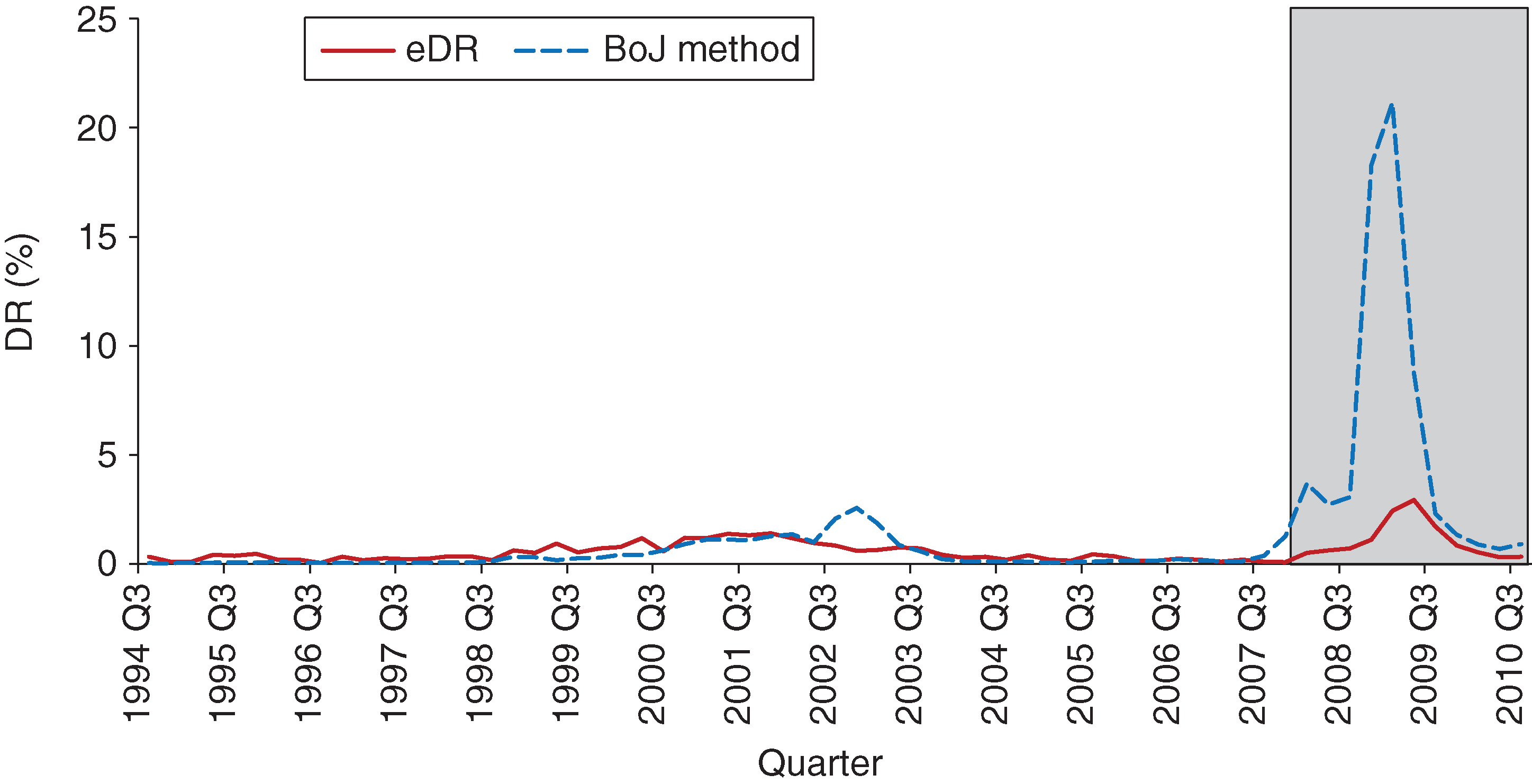
The most striking observation from Figure 14 is that in the out-of-sample testing period the estimated DRs are significantly larger than the actual DRs. We believe the reason for this gap lies in the fact that the method is not designed to handle large numbers of zero entries in the TPM. Such large numbers of zero entries adversely affect the regression models used in the computation of the DR.
We took the method in Otani et al (2009) one step further and applied a smoothing algorithm to fill in the zero TPM entries across the rows. This means that, after applying the smoothing, the zero entries are replaced by strictly positive, very small numbers. The in-sample and out-of-sample results after applying the smoothing are presented in Figure 15.

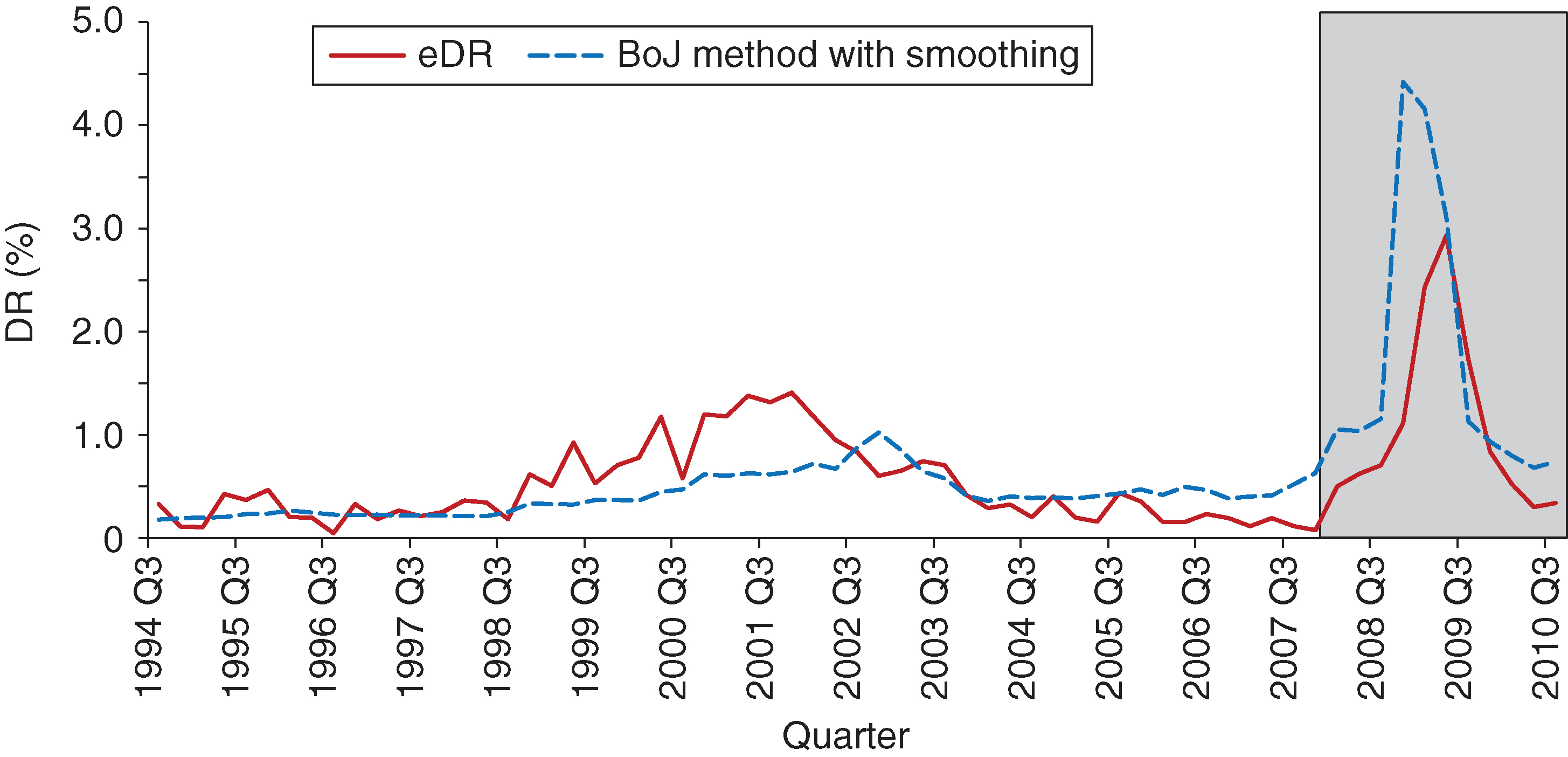
It is obvious the results have improved dramatically after applying the smoothing. There is much better agreement, out-of-sample in particular, between the estimated DR and the actual DR. The in-sample performance of this method is not as good as for the other two presented earlier. In particular, it performs quite poorly during the 2001 dot-com bubble; neither the level nor the timing of that episode is accurately captured. Out-of-sample, the maximum difference between the projected DR and the actual DR is 1.49%, the mean absolute error is 0.74% and the sum of squared errors is 0.16%. As is the case with the other methods, the DR estimate is higher than the actual DR in the out-of-sample period.
5 Results comparison
In this section, we summarize results from the three methods presented in this paper: our proposed BI method, Moody’s method and that of Otani et al (2009) from the Bank of Japan. These are the same results presented in previous sections; here, however, we showcase them simultaneously and contrast their performance in- and out-of-sample.
Figure 16 shows the in- and out-of-sample fits for the three methods, overlaid together.

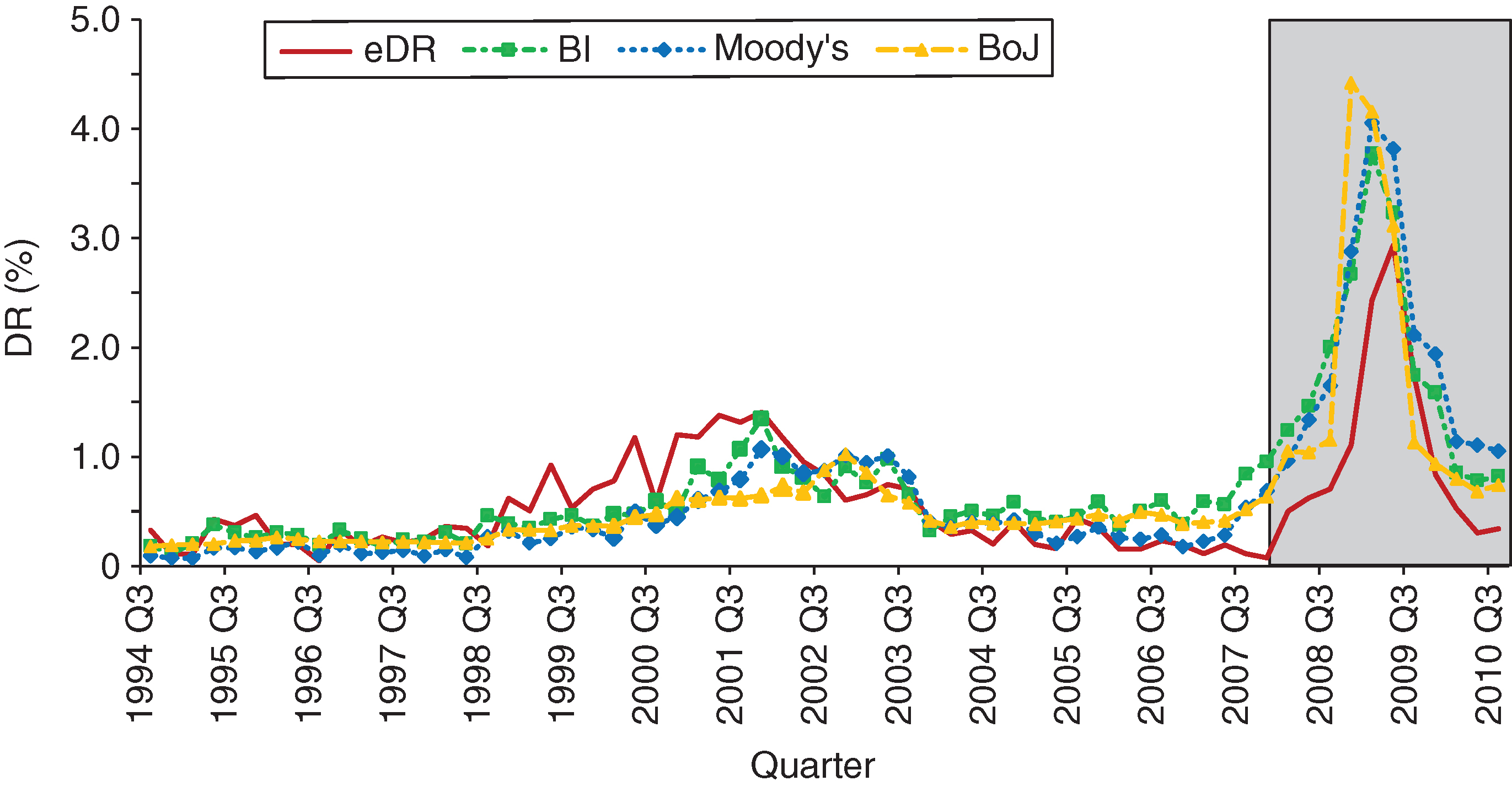
In Figure 16, we see that, out-of-sample, all methods are conservative, in the sense that they all project a higher DR than the actual DR observed in the data. Overall, we think the BI method performs better than the other two, although Moody’s method is not far off. We consider two main criteria when making this assessment: the timing of the projected peak and both the speed and the level for the recovery post-peak. Of course, other criteria metrics might single out different methods as being preferable: for example, the Bank of Japan method gives the best mean absolute error (however, the timing and magnitude of the peak are most off for this method compared with the other two; see discussion below). All anticipate the peak in DR well, with the BI method projecting more conservative DRs during the initial part of the out-of-sample period (2007 Q4–2008 Q2). The Bank of Japan method is the most off in terms of timing the 2009 Q2 peak in DR, with the BI method having the most accurate timing (although the differences are not likely to be of statistical significance). The BI and Bank of Japan methods have the closest-to-actual DR decline post the 2009 Q2 peak, both in terms of speed of recovery and the levels projected. Moody’s method is the slowest to react: the level of projected DR hovers around 1.05% in 2010 Q3 for this method, while the actual DR is 0.34%; the other two methods predict 0.82% (BI) and 0.74% (Bank of Japan).
In-sample, the story is somewhat mixed, and conclusions are again dependent on the assessment criteria. For the 2001 dot-com bubble, the BI method performs best out of the three. It very accurately matches the 2001 Q4 peak (from both a level and a timing perspective): the actual DR is 1.41% and the BI method projects a 1.35% DR. It also recovers well (in terms of speed as well as level) post this peak, matching very closely the actual DR of 0.42% in 2003 Q4 (the projected value is 0.32%). The other two methods do not perform as well during this time period. Moody’s method does have good timing in terms of matching the 2001 Q4 peak, but the level is off: it projects a 1.07% DR for 2001 Q4. It is also slow to recover post-peak, projecting DR at roughly the same level until 2003 Q2 before dropping in value. Both timing and level are off for the Bank of Japan method, which is the weakest performer of the three. For the time period leading up to the 2001 Q4 peak, all methods predict lower DR than the DR observed in the data. Leading up to the end of the training sample, Moody’s method follows the actual DR closest, with the BI and Bank of Japan methods projecting higher DR (the BI method projects the highest).
6 Conclusion
In this paper, we present a method, which we call the BI method, for credit portfolio stress testing using transition probability matrixes. We contrast results from this proposed method with results obtained from two competing approaches: Moody’s method, as detailed in Licari et al (2013), and the Bank of Japan method, as detailed in Otani et al (2009). This benchmarking study is done out-of-sample, where the validation set is chosen to coincide with the time frame of the 2008 financial crisis; it therefore provides an accurate proxy for a stressed environment.
All three methods presented here follow a common approach. Each extracts certain features from the transition probability matrix, performs regression analysis to connect these features to macroeconomic variables, and uses forecasted stressed values of these variables to project stressed transition probability matrixes and so compute the implied stressed default rates. The BI method relies on bias and inertia as features to be extracted; Moody’s method relies on the principal components of the one-notch and two-notch transitions; and the Bank of Japan method relies on the factors that combine rating-specific information () with systemic information (). From the results and discussion in Section 5, we see that the BI method has a slightly better performance out-of-sample (with Moody’s method a close second), while in-sample it performs better during the 2001 dot-com bubble but lags behind the other two methods over the period leading up to the 2008 financial crisis. Both the BI and Moody’s methods outperform the Bank of Japan method overall. The BI method is also simpler, the number of key drivers required being two (bias, inertia), while for Moody’s method this equals the number of principal components chosen. In practice, we found that at most three principal components are needed for upgrades, downgrades, and one-notch and two-notch transitions, respectively; hence, a total of approximately twelve drivers.
As far as future work is concerned, we can ask the question of whether working with just two key drivers is not oversimplifying reality and therefore potentially creating limitations. We showed that bias and inertia already carry substantial information in characterizing the transition probability matrix, but augmenting them with additional information would probably do an even better job of describing the transition matrixes. A few suggestions are as follows: introducing some level of segmentation/block pattern when thinking about how to capture the upgrade/downgrade mass in a transition matrix, or using information beyond the main diagonal when trying to assess the level of mobility. Another item for future study is the collapsing of grades, especially if dealing with high credit quality portfolios. The segmentation/block pattern idea mentioned above could also be applicable here. Finally, improving on the regression models that link the key transition probability matrix drivers to the macroeconomic variables is also an area that could benefit from further study.
Declaration of interest
The authors report no conflicts of interest. The authors alone are responsible for the content and writing of the paper.
References
- Arvanitis, A., Gregory, J., and Laurent, J.-P. (1999). Building models for credit spreads. Journal of Derivatives 6(3), 27–43 (https://doi.org/10.3905/jod.1999.319117).
- Bangia, A., Diebold, F. X., Kronimus, A., Schagen, C., and Schuermann, T. (2002). Ratings migration and the business cycle, with application to credit portfolio stress testing. Journal of Banking & Finance 26, 445–474 (https://doi.org/10.1016/S0378-4266(01)00229-1).
- Belkin, B., Suchower, S., and Forest, L. (1998). A one-parameter representation of credit risk and transition matrices. Creditmetrics Monitor, Third Quarter, 46–58.
- Belotti, T., and Crook, J. (2009). Credit scoring with macroeconomic variables using survival analysis. Journal of the Operation Research Society 60(12), 1699–1707 (https://doi.org/10.1057/jors.2008.130).
- Carling, K., Jacobson, T., Linde, J., and Roszbach, K. (2007). Corporate credit risk modeling and the macroeconomy. Journal of Banking and Finance 31(3), 845–868 (https://doi.org/10.1016/j.jbankfin.2006.06.012).
- Fons, J. S. (1991). An approach to forecasting default rates. Special Report, Moody’s Investor Services.
- Frydman, H., and Schuermann, T. (2008). Credit rating dynamics and Markov mixture models. Journal of Banking & Finance 32(6), 1062–1075 (https://doi.org/10.1016/j.jbankfin.2007.09.013).
- Hanson, S., and Schuermann, T. (2006). Confidence intervals for probabilities of default. Journal of Banking & Finance 30, 2281–2301 (https://doi.org/10.1016/j.jbankfin.2005.08.002).
- Inamura, Y. (2006). Estimating continuous time transition matrices from discretely observed data. Working Paper, Bank of Japan.
- Jafry, Y., and Schuermann, T. (2003). Metrics for comparing credit migration matrices. Working Paper 03-09, Wharton Financial Institutions Center (https://doi.org/10.2139/ssrn.394020).
- Jafry, Y., and Schuermann, T. (2004). Measurement, estimation and comparison of credit migration matrices. Journal of Banking & Finance 28, 2603–2639 (https://doi.org/10.1016/j.jbankfin.2004.06.004).
- Keenan, S., Li, D., Santilli, S., Barnes, A., Chalermkraivuth, K., and Neagu, R. (2008). Credit cycle stress testing using a point in time rating system. In Stress Testing for Financial Institutions: Applications, Regulations and Techniques, Rösch, D., and Scheule, H. (eds), pp. 37–66. Risk Books, London.
- Koopman, S. J., and Lucas, A. (2005). Business and default cycles for credit risk. Journal of Applied Econometrics 20, 311–323 (https://doi.org/10.1002/jae.833).
- Koopman, S. J., Lucas, A., and Monteiro, A. (2008). The multi-state latent factor intensity model for credit. Journal of Econometrics 142, 399–424 (https://doi.org/10.1016/j.jeconom.2007.07.001).
- Lando, D., and Skødeberg, T. M. (2002). Analyzing rating transitions and rating drift with continuous observations. Journal of Banking & Finance 26, 423–444 (https://doi.org/10.1016/S0378-4266(01)00228-X).
- Licari, J. M., Suárez-Lledó, J., and Black, B. (2013). Stress testing of credit migration: a macroeconomic approach. Report, Moody’s Analytics.
- Long, K., Keenan, S. C., Neagu, R., Ellis, J. A., and Black, J. W. (2011). The computation of optimised credit transition matrices. Journal of Risk Management and Financial Institutions 4(4), 370–391.
- Miu, P., and Ozdemir, B. (2009). Stress testing probability of default and rating migration rate with respect to Basel II requirements. The Journal of Risk Model Validation 3(4), 3–38 (https://doi.org/10.21314/JRMV.2009.048).
- Nickell, P., Perraudin, W., and Varotto, S. (2000). Stability of rating transitions. Journal of Banking & Finance 24, 203–227 (https://doi.org/10.1016/S0378-4266(99)00057-6).
- Okashima, K., and Fridson, M. (2000). Downgrade/upgrade ratio leads default rate. Journal of Fixed Income 10(2), 18–24 (https://doi.org/10.3905/jfi.2000.319267).
- Otani, A., Shiratsuka, S., Tsurui, R., and Yamada, T. (2009). Macro stress-testing on the loan portfolio of Japanese banks. Working Paper, Bank of Japan.
- Perilioglu, A., Perilioglu, K., and Tuysuz, S. (2018). A risk-sensitive approach for stressed transition. The Journal of Risk Model Validation, Online Early (https://doi.org/10.21314/JRMV.2018.192).
- Skoglund, J. (2017). Forecast of forecast: an analytical approach to stressed impairment forecasting. Journal of Risk Management in Financial Institutions 10(3), 238–256 (https://doi.org/10.2139/ssrn.2902565).
- Sobehart, J. (2008). Uncertainty, credit migration, stressed scenario and portfolio losses. In Stress Testing for Financial Institutions: Applications, Regulations and Techniques, Rösch, D., and Scheule, H. (eds), pp. 197–237. Risk Books, London.
- Sobehart, J., and Keenan, S. (2004). Modeling credit migration for credit risk capital and loss provisioning calculations. RMA Journal, October, 30–37.
- Sobehart, J., and Sun, X. (2018). A foundational approach to credit migration for stress testing and expected credit loss estimation. Journal of Risk Management in Financial Institutions 11(2), 156–172.
- Trück, S. (2004). Measures for comparing transition matrices from a value-at-risk perspective. Working Paper, Institute of Statistics and Mathematical Economics, University of Karlsruhe.
- Trück, S. (2008). Forecasting credit migration matrices with business cycle effects: a model comparison. European Journal of Finance 5(14), 359–379 (https://doi.org/10.1080/13518470701773635).
- Wei, J. Z. (2003). A multi-factor, credit migration model for sovereign and corporate debts. Journal of International Money and Finance 22, 709–735 (https://doi.org/10.1016/S0261-5606(03)00052-4).
- Yang, H. B. (2017). Forward ordinal probability models for point-in-time probability of default term structure: methodologies and implementations for IFRS 9 expected credit loss estimation and CCAR stress testing. The Journal of Risk Model Validation 11(3), 1–18.
- Zhang, J., Avasarala, V., and Subbu, R. (2010). Evolutionary optimization of transition probability matrices for credit decision-making. European Journal of Operational Research 200, 557–567 (https://doi.org/10.1016/j.ejor.2009.01.020).
Only users who have a paid subscription or are part of a corporate subscription are able to print or copy content.
To access these options, along with all other subscription benefits, please contact info@risk.net or view our subscription options here: http://subscriptions.risk.net/subscribe
You are currently unable to print this content. Please contact info@risk.net to find out more.
You are currently unable to copy this content. Please contact info@risk.net to find out more.
Copyright Infopro Digital Limited. All rights reserved.
As outlined in our terms and conditions, https://www.infopro-digital.com/terms-and-conditions/subscriptions/ (point 2.4), printing is limited to a single copy.
If you would like to purchase additional rights please email info@risk.net
Copyright Infopro Digital Limited. All rights reserved.
You may share this content using our article tools. As outlined in our terms and conditions, https://www.infopro-digital.com/terms-and-conditions/subscriptions/ (clause 2.4), an Authorised User may only make one copy of the materials for their own personal use. You must also comply with the restrictions in clause 2.5.
If you would like to purchase additional rights please email info@risk.net