Journal of Risk
ISSN:
1755-2842 (online)
Editor-in-chief: Farid AitSahlia
An internal default risk model: simulation of default times and recovery rates within the new Fundamental Review of the Trading Book framework
Andrea Bertagna, Dragos Deliu, Luca Lopez, Aldo Nassigh, Michele Pioppi, Fabian Reffel, Peter Schaller and Robert Schulze
Abstract
In January 2016, the Basel Committee on Banking Supervision published its new requirements for the calculation of market risk within the banking sector. These requirements go under the name of the Fundamental Review of the Trading Book. The default risk model is one part of these requirements that is subject to material changes: recovery rates must be stochastic variables, basis risk due to differences in recoveries have to be considered, and a dependence between recovery rates and systematic risk factors used to simulate default times must be enforced. This paper presents a new default risk model for market risk that is consistent with these requirements. The recovery rates follow a waterfall model that is based on a minimum entropy principle. Moreover, the model features correlation between default times and stochastic recovery rates by exploiting the observed correlation between default frequency and average recoveries in historical data. As well as giving some mathematical background, the authors present the numerical results and the impacts of the various model parameters. These show that the introduced correlation can have a significant impact on the capital charge.
Introduction
Abstract
In January 2016, the Basel Committee on Banking Supervision published its new requirements for the calculation of market risk within the banking sector. These requirements go under the name of the Fundamental Review of the Trading Book. The default risk model is one part of these requirements that is subject to material changes: recovery rates must be stochastic variables, basis risk due to differences in recoveries have to be considered, and a dependence between recovery rates and systematic risk factors used to simulate default times must be enforced. This paper presents a new default risk model for market risk that is consistent with these requirements. The recovery rates follow a waterfall model that is based on a minimum entropy principle. Moreover, the model features correlation between default times and stochastic recovery rates by exploiting the observed correlation between default frequency and average recoveries in historical data. As well as giving some mathematical background, we present the numerical results and the impacts of the various model parameters. These show that the introduced correlation can have a significant impact on the capital charge.
1 Introduction
In January 2016, the Basel Committee on Banking Supervision (2016) revised the standards for the minimum requirement for market risk (Fundamental Review of the Trading Book (FRTB)), and these standards will replace the current framework, which is known as Basel 2.5. Three years later, in January 2019, the Basel Committee on Banking Supervision (2019) published the final framework, which serves as a basis for the various jurisdictions around the world for transposition into local law. All affected banks in every jurisdiction have to comply with these rules and thereby preserve a certain capital buffer for the positions held on their books.
The framework consists of two parts: a mandatory standardized approach (SA) based on prescribed regulatory rules, and an internal models approach (IMA) that allows banks to use more sophisticated models, provided they comply with a given set of requirements. Moreover, a specific percentage of the capital requirement stemming from the SA serves as a floor for the capital charge coming from the IMA.
The IMA capital charge is made up of three components: an expected shortfall model that is meant to cover losses arising from historical movements of market variables with a sufficient number of observations in the last year; a model that covers the remaining market variables; and a default risk charge (DRC). The DRC is meant to cover losses arising from issuers’ defaults, ie, those losses that are not captured by the credit spread volatility in the expected shortfall model. The DRC will replace the current incremental risk charge (IRC) that, besides defaults, also embeds losses coming from migration events. While the removal of rating migrations simplifies the calculations, the mandatory requirements from the FRTB potentially complicate the model compared with the IRC. Specifically, the main requirements that the DRC model must comply with are as follows.
- (1)
Besides credit products, the simulation must also include equity instruments.
- (2)
Basis risks due to differences in recoveries for securities issued from the same obligor must be considered.
- (3)
Maturity mismatches between a position and its hedge must be taken into account.
- (4)
In addition to credit spreads, equity spot prices must also be used to determine default correlations.
- (5)
Recovery rates (RRs) must be stochastic variables.
- (6)
The internal default risk model must include the dependence between RRs and systematic risk factors used to simulate default times.
This paper describes an algorithm for the DRC calculation that copes with these regulatory requirements, with a special focus on points (2), (5) and (6). The other requirements are naturally embedded in our model but are not discussed in detail in this paper. Indeed, the jump-to-default (JTD) values for equities are simply included in the scope, the maturity mismatch is accounted for in the explicit simulation of default times and the default correlations are supposed to be external model inputs.
However, given its relevance, the calibration of default correlations (point (4)) deserves some discussion. Solutions to this problem can be classified according to two approaches. The first involves deriving the default correlation via maximum likelihood (ML) from the time series analysis of past defaults on representative portfolios, as recently performed in Chava et al (2011). An extensive survey of methodologies based on ML estimation is given in Altman (2008). In the second approach, default correlations can be derived from market data, following the methodology first introduced in the 1990s with CreditMetrics (JP Morgan 1997).
Derivation of the default correlation via ML has the obvious advantage of being the most straightforward way to infer from time series analysis the variable under consideration, ie, the correlation among actual defaults. The disadvantage of this approach is that default is, in general, a rare event. As a consequence, in order to be statistically significant, the ML estimation must be applied to a large sample of firms observed over a multiyear period. As a matter of fact, it is very difficult to build a sufficiently large database with proprietary data within a single financial institution, and the analyst must therefore resort to large, publicly available databases based on rating agency data, such as Moody’s Ultimate Recovery Database, for example.11 1 See http://www.moodys.com/Pages/Default-and-Recovery-Analytics.aspxformoredetails. However, usage of rating agency data is an effective way of deriving the loss distribution for credit portfolios whose issuers have access to the capital market (for debt instruments), which are quite different from the typical credit portfolio of a bank, particularly in Europe. On top of that, the vast majority of default events recorded by rating agencies are related to sub-investment-grade issuers, and this also calls into question the representativeness of the correlation estimations when they are applied to credit portfolios that are mainly exposed to investment-grade names, which is the case for portfolios subject to the DRC.
For the two reasons given above, derivation from market data following CreditMetrics is now widespread within the financial industry for credit value-at-risk models. Such an approach has the obvious disadvantage that the default correlation is derived from proxies: the correlation between equities (or credit default swaps) is a proxy for asset correlations, which are, in turn, proxies for default correlations.
Coming to the main points of the paper, requirement (2) is achieved via a waterfall mechanism that accounts for three different seniorities. Requirements (5) and (6) are the most demanding since they ask for a dependency between simulated defaults and recoveries. How to model this dependency is still an open topic that is subject to investigation by analysts from both industry and academia. The Basel Committee on Banking Supervision (2016) does not prescribe any explicit model: it simply requires banks to reflect the economic cycle in their loss estimates.
The first open issue in the debate concerns the economic reasons for the observed dependence between default frequency (DF) and loss given default (LGD). This can be grounded in the fluctuations of the value of the firm asset used as collateral to pay back creditors after bankruptcy. Following this approach, Frye (2000a, b) developed a model in which the realized RR is driven by the same macrofactor that drives the firm’s probability of default (PD). This is a single-factor model that extends the asymptotic single risk factor model introduced by Gordy (2003) to the stochastic RR case; this is now embodied in the risk weight formula of the Basel II regulations from the Basel Committee on Banking Supervision (2005).
Taking an alternative approach, Altman et al (2002) derive the dependency between DF and LGD on the basis of a supply-and-demand argument. Indeed, they observe that the market for defaulted debt lacks breadth. As a consequence, in years of high DF the market price of defaulted securities (the so-called market recovery rate, or market RR) is depressed because of the increased offer. Under the latter approach, we should observe a lower dependency between DF and LGD when the “workout recovery rate” (workout RR) is considered, ie, the value of the actual recoveries gathered by the holder of the defaulted debt in the months (or years) after the default, discounted at the time of default.
Workout RR is more difficult to estimate than market RR, and indeed most of the data published by rating agencies concerns the latter. However, Düllmann and Gehde-Trapp (2004) were able to compare the two measures and found that the dependency between DF and LGD is much less significant if workout RR is considered. They measured the correlation between DF and RR via ML on a representative portfolio of defaulted debt and found a less significant -value and a smaller absolute value of the correlation.22 2 The positive dependence between DF and LGD is reflected in a negative correlation between DF and RR since, in general, . In particular, they found that the hypothesis of nonzero correlation is significant at the 99% level only if the market RR is considered.
This latter result could explain the difference between the position taken by the regulators regarding the minimum capital requirement for credit risk, ie, the usage of a stressed LGD, and the requirement set forth for the DRC in the trading portfolio: namely, the request for a full simulation. The economic losses of the credit portfolio of a representative bank will be driven by the price of the defaulted firm’s assets at the start of the recovery process. Conversely, the bank is expected to cash in securities in the trading book in the aftermath of the default, and the economic loss will therefore be determined by the level of the market RR.
The models developed by Frye (2000b), Pykhtin (2004) and Düllmann and Gehde-Trapp (2004) belong to the single-factor family. However, the DRC must be calculated according to a multifactor model, in keeping with the current best practice for IRC models. Acharya et al (2007) and Varma and Cantor (2005) analyzed the linear multifactor dependence of creditor recoveries. Later, Chava et al (2011) estimated the coefficients of alternative multifactor models for the forecast of the loss distribution via ML on representative portfolios of defaulted debt. These models take into account both stochastic PD and stochastic RR. Their results confirm the materiality and statistical significance of a negative correlation between DF and market RR as already shown in the single-factor models and in the empirical analysis of Altman et al (2005).
The algorithm proposed in this paper relies on the above results and is tailored for implementation, risk management and measurement purposes. It consists of four steps.
- •
In the first step, we define so-called fundamental risk factors that serve as systemic drivers.
- •
In the second step, correlated default times are simulated via a copula, eg, a Gaussian or Student copula.
- •
In the third step, DF and RR are simulated and correlated to the default times.
- •
Finally, the data is combined with the JTDs.
2 The algorithm
This section describes the steps of the algorithm that underlies our DRC model. Mathematical details and additional information are provided in the online appendix.
2.1 Fundamental risk factors
First of all, we select a given number of predefined risk factor time series that are supposed to represent the whole market. A risk factor time series could be a credit spread for a given maturity of a specific company over a certain time period, eg, the five-year pillar for the Google credit default swap curve from 2007 to 2017 as a representative of a technology company. From these risk factor time series, nonoverlapping normalized ten-day returns are calculated. The return calculation depends on the risk factor type: differences for credit risk factors and log returns for equities. In order to have homogeneous variables, returns are normalized by the standard deviation.
These normalized returns are used as explanatory variables in the regression on the individual issuer’s time series. In order to improve the robustness and stability of the regression, we first perform a principal component analysis (PCA) and select the first components that explain a sufficient portion of the variability of the original returns. These components represent the fundamental risk factors (FRFs) entering the model.
2.2 Simulation of correlated default times
We now focus on the actual issuers to be simulated. Again, we determine for each issuer a risk factor time series and calculate the respective normalized returns. We then perform a linear regression of the normalized returns on the FRFs with zero intercept. This gives us a set of coefficients for each issuer :
| (2.1) |
We model the default time for the issuer assuming an exponential distribution for the default times. The rate parameter is calibrated to the issuer’s one-year PD. To model the dependence on the FRFs, a copula method is applied. A discussion about the use of different copulas (Gaussian, Student , Clayton) and their impact on DRC is given in Wilkens and Predescu (2017). That study reveals that for diversified portfolios, the capital impact of different copulas is around 10%. Our proposed method for the default time and RR simulation is not dependent on the chosen copula, ie, the copula can be exchanged easily with very few adaptations, none of which affect parts of the method other than the default time simulation itself. To keep it simple, we select the Gaussian copula. (For a discussion on extending this to a Student copula, see Appendix C online.) We then have
| (2.2) | ||||
| where | ||||
| (2.3) | ||||
is the cumulative standard normal distribution, is the one-year PD for issuer , and and are independent normal standard variables. Appendix C (online) offers a more detailed explanation and gives the motivation for the formulas.
2.3 Simulation of RRs
2.3.1 The waterfall mechanism for RRs
Our waterfall model has three main characteristics. First, three different seniorities are taken into account. Second, the RRs are simulated according to a minimum entropy distribution. This distribution has two main features.
- •
The density distribution is positive at zero and one, so RRs close to the boundaries have a nonzero probability. This is in line with historical data.
- •
The minimum entropy distribution comes with a theoretical framework that allows the waterfall parameters to be constrained easily.
Third, the dependence between defaults and RRs is induced via a rank correlation mechanism that can be calibrated to historical data. This reveals that the number of defaults and the LGD are usually positively correlated.
A more detailed discussion about the properties of the minimum entropy distribution to simulate RRs can be found in Schaller (2018).
2.3.2 The waterfall model in detail
Our model assumes four types of issues subject to different recoveries:
- (1)
secured debt,
- (2)
senior unsecured debt,
- (3)
subordinated debt and
- (4)
equity.
In addition, we assume that the recovery process can be generalized as follows.
- •
All secured issues have the same RR. This is the case, for example, if they are linked to the same collateral pool and no subordination between secured issues is defined.
- •
There is only one level of subordination between unsecured issues.
- •
Subordinated debt has a nonzero RR only if senior debt fully recovers.
- •
Equity always yields zero RR as required by the Basel Committee on Banking Supervision (2016, Section 186(c)).
In the case of the default of an issuer, the RRs are linked by the following waterfall mechanism. The collateral allocated to the secured debt is used to pay back the secured debt. The remaining secured debt is then treated as senior unsecured debt. The remaining assets of the issuer are then used to pay back the senior unsecured debt. After all of the senior unsecured debt has been paid back, remaining assets are used to pay back the subordinated debt. Finally, the RR on the equity tranche is forced to be , although, in practice, any assets that remain after this step would be distributed to the equity holders. In the case where the collateral associated with the secured tranche is not enough to repay the secured debt, the assets associated with the unsecured tranche are also used to repay part of the outstanding secured debt. The RR of this portion of the secured debt is equal to the RR of the unsecured tranche.
The inputs for the model are the expected RRs per issuer and having seniority . The realizations of the RRs are denoted by lowercase letters. According to our assumptions from above, the RRs are ordered such that , and they are therefore the expected RRs. To get rid of this dependency, conditional expected RRs are used. That is:
- (1)
is the expected portion of secured debt covered by the collateral;
- (2)
is the expected portion of senior unsecured debt covered by the remaining assets of the issuer on the condition that the subordinated debt has zero recovery;
- (3)
is the expected portion of subordinated debt covered by the remaining assets of the issuer on the condition that the senior unsecured debt has full recovery; and
- (4)
the probability of the senior unsecured debt having full recovery is .
The expected RRs are connected. The RR of the secured tranche is the portion of secured debt covered by associated collateral plus the RR of the senior tranche for the portion of the secured debt not covered by the collateral, ie,
| (2.4) |
The expected value of the RR for the senior unsecured tranche, , is the probability-weighted sum of both the event that the senior unsecured tranche is fully recovered and the conditional recovery of the senior tranche given that the remaining assets of the borrower do not suffice to fully recover the senior unsecured tranche, ie,
| (2.5) |
The subordinated tranche recovers only in the event that the senior unsecured tranche fully recovers. Thus, we have
| (2.6) |
We solve these equations for in order to calculate the mean of the conditional expected RRs as a function of for . Consequently, we need a fourth equation. This equation is retrieved from the minimum entropy principle, details about which are given in Appendix D online. The resulting relation is
| (2.7) |
Thus, we have four variables, , , , , and four equations (2.4), (2.5), (2.6) and (2.7). Solving these for , and gives
| (2.8) | ||||
| (2.9) | ||||
| (2.10) |
To simulate the realized recoveries , and for issuer and for the three different types of issues (senior secured, senior unsecured, subordinated), we need the following random variables.
- (1)
A bivariate variable , taking the value if there is a nonzero recovery for subordinated debt (ie, with probability ) and otherwise.
- (2)
A variable with mean on the interval for the portion of secured debt covered by the associated collateral.
- (3)
A variable with mean on the interval for the conditional recovery of the senior unsecured debt in the case it does not fully recover.
- (4)
A variable on the interval with mean describing the conditional realized recovery for the subordinated debt when it is nonzero.
From the minimum entropy principle, we can conclude that the variables and are distributed according to an exponential distribution on that is fully determined by its mean. is also distributed according to an exponential distribution on ; this can be seen in Appendix D.3 (online) as a simplified case of and .
The algorithm for the simulation of the RRs is then the following:
| (2.11) | ||||
| (2.12) | ||||
| (2.13) | ||||
| (2.14) |
From this, is a realization of the random variable , is a realization of the random variable , and likewise for and .
2.3.3 Correlation between default times and RRs
If an economy is in a downturn, the defaulted companies cannot rely on other companies to take them over or on a government bailout. Hence, the simultaneous defaults of multiple issuers usually go hand in hand with low RRs, especially for the unsecured tranches. In this paper’s introduction we provided further explanation and referenced relevant literature to underpin this observation. Therefore, we introduce a dependency between the DF and the unsecured RRs. More precisely, we correlate the number of defaults in a scenario with the sum of the senior unsecured and the subordinated . This dependence is achieved via a rank correlation between the number of issuers that default in less than a year and the simulated LGDs. This rank correlation is induced via an order map that is used to align the ordering of the number of defaults in scenario with the ordering of the sum of the respective LGDs for that issuer . Details about the method for computing a rank correlation between two distributions are given in Appendix E online.
The level of correlation is an exogenous parameter and significantly affects the order map. In particular, if , the map induces the exact same ordering between LGD and DF. This means that scenarios with the highest numbers of defaults are those with the highest aggregated LGDs. This represents the most punitive scenario for the bank. At the other extreme, with , the map induces a reverse ordering, giving rise to milder default losses. Any sits between these two extreme variants and therefore establishes a correlation between the number of simultaneous default events and the level of LGDs. In the special case , DF and LGD are uncorrelated.
2.3.4 Calibration of rank correlation
One of the most relevant aspects of the proposed model is the possibility of calibrating the issuer’s rank correlation , introduced in Section 2.3.3 to historical data. Several rating agency databases store information about both historical default events and RRs. The default event information is used to obtain the DF while the RR information is used to compute the average LGD. The rank correlation between DFs and the sum of the average LGD is quantified via Spearman’s rank correlation coefficient. It is worth noting that the correlation between the average LGD and the DF is higher than that between the LGD of the individual issuer and the DF. This can be inferred by considering the case of normally distributed variables. If variables have an independent idiosyncratic component and have a correlation with a given variable , ie, , then the sum has a correlation with , which is given by
| (2.15) |
This framework is used to approximate the single issuer correlation given the correlation between the DF and the average LGD:
| (2.16) |
where and are proxies for and , respectively, and is the average number of yearly defaults.
2.4 Aggregation and DRC computation
For each scenario, and for each instrument with at least one defaulting underlying issuer in the given scenario, ie, underlying issuers with default times not greater than the instrument’s maturity, a JTD value has to be calculated. The calculation depends on the instrument’s seniority and the simulated RR. The JTD in each scenario is given by the sum of JTDs of the individual instruments. According to the FRTB, the 99.9% quantile of the JTD distribution corresponds to the DRC.
3 Examples
The performance of the proposed simulation scheme is numerically assessed in terms of capital charge for a hypothetical portfolio. In Section 3.1 the exercise setup is described, while results are reported and discussed in Section 3.2.
3.1 The setup of the example
3.1.1 Choice of FRFs
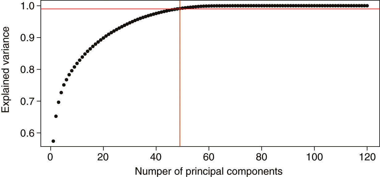
According to the regulations, two types of FRFs must be used. To comply with the rules, credit spread indexes for different sector–rating combinations and country (or region) equity indexes are used as FRFs. Beyond the obvious differences between spreads and equities, such typologies capture different sources of correlations among issuers: spreads reflect the affiliation of issuers to the same sector–rating combination, while equities are more related to the issuer region. In this example, from an initial list of 120 FRFs composed of around forty equity indexes from the most relevant markets and eighty generic credit spreads, about fifty components are selected via PCA. These components cover more than 99% of the system variance (see Figure 1).

3.1.2 Choice of time interval
Regulations insist that we use at least ten years’ worth of time series to calibrate the model. For the choice of the length of the return calculation , ten days is deemed to be a good compromise between the needs of the regulations and the accuracy of the estimation of regression parameters.
3.1.3 Choice of hypothetical portfolio of issuers

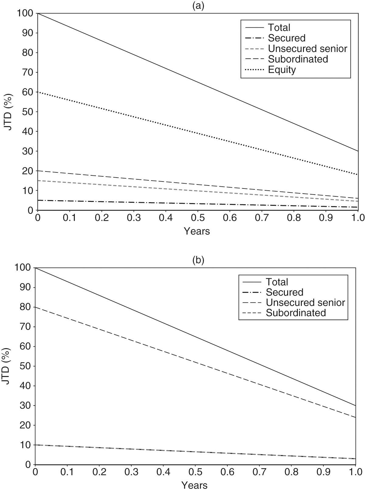
The hypothetical portfolio has been designed in such a way that it has an overall exposure that is split equally between corporates and sovereigns. The JTD of corporates is dominated by equity, while exposures to sovereigns are driven by unsecured senior bonds. This hypothetical portfolio has the following peculiarities.
- •
There are 5000 corporate issuers.
- –
The JTD of corporates is linearly distributed between million and million. If an issuer has a negative JTD value, the bank realizes a profit when the issuer defaults.
- –
The JTD of each corporate has the following composition:
- *
5% secured debt,
- *
15% unsecured senior debt,
- *
20% subordinated debt, and
- *
60% equity.
- *
- –
- •
There are 100 sovereign issuers.
- –
The JTD of the sovereign is linearly distributed between million and million.
- –
The JTD of each corporate has the following composition:
- *
10% secured debt,
- *
80% unsecured senior debt, and
- *
10% subordinated debt.
- *
- –
- •
The average correlation among issuer default times is slightly above 20%.
- •
The average idiosyncratic component in the simulation of default times is 50%.
- •
The default probability of each issuer in the first year is 0.5%.
- •
The RR of each issuer for the equity component is .
- •
The average RR of each issuer for the secured component of the debt is 0.8.
- •
The average RR of each issuer for the senior unsecured component of the debt is 0.4.
- •
The average RR of each issuer for the subordinated component is 0.2.
- •
Each issuer reduces its JTD linearly in time, with a decrease of 70% after the first year (Figure 2).
The level of rank correlation between the DF and the average LGD varies between 0% and 100%, and the results are computed for all the configurations.

3.2 Results and discussion
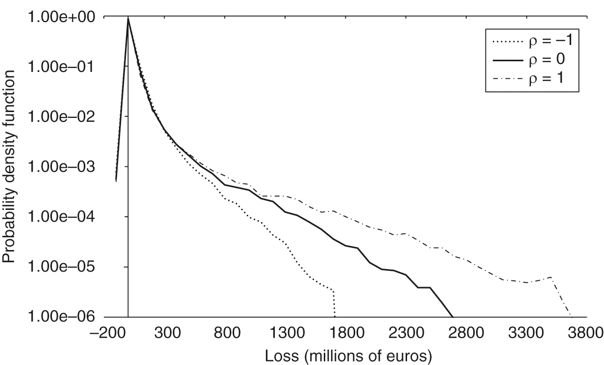
The presence of a rank correlation between the DF and the LGDs affects the loss distribution of the bank. In Figure 3, three extreme cases () are shown. As expected, when the tails of the loss distribution are more pronounced, while in the absence of correlation the loss tends to be reduced and to have a concentration around 0. The reduction of the right tail is amplified when correlation is negative. The distribution is asymmetric because of the test setup, where losses are favored with respect to gains.
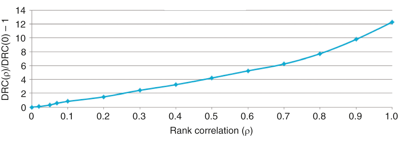
From a risk perspective, the cases where high frequency corresponds to a low RR () are the most relevant. The impact of rank correlation on the charge distribution is shown in Figure 4, where the increase in DRC with respect to the uncorrelated case is presented. As expected, the DRC is a monotonic function of , with an increase of 2% for and 12% for .

4 Conclusion
The new requirements for the capitalization of default risk in the trading book pose some methodological challenges and demand a departure from the current IRC model. In particular, the simulation of default times (to properly take into account possible maturity mismatches between a position and its hedge) and RRs, and the dependence between RRs and the systemic risk factors, are some of the key ingredients that a new internal default risk model is supposed to embed. A model that fully complies with these new requirements is proposed. Default times are simulated via a Gaussian copula, and a rank correlation between the DF and the average LGD is imposed in order to reflect the economic cycle in the loss estimates. The level of correlation is an exogenous parameter of the model, and an algorithm to calibrate the proposed model to is described. The impact of the rank correlation between default times and LGD has been assessed via a numerical example. As expected, the DRC is a monotonic function of correlation, the highest value occurring when the DF and the average LGD are fully correlated, ie, is set to . The increase in the charge when moving from the uncorrelated case to the fully correlated case is slightly above 10%.
Declaration of interest
All authors are employed by UniCredit SpA or its legal entities. The views, thoughts and opinions expressed in this paper are those of the authors in their individual capacities and should not be attributed to UniCredit group or to the authors as representatives or employees of UniCredit group. The authors report no conflicts of interest. The authors alone are responsible for the content and writing of the paper.
References
- Acharya, V. V., Bharath, S. T., and Srinivasan, A. (2007). Does industry-wide distress affect defaulted firms? Evidence from creditor recoveries. Journal of Financial Economics 85(3), 787–821 (https://doi.org/10.1016/j.jfineco.2006.05.011).
- Altman, E. I. (2008). Default recovery rates and LGD in credit risk modeling and practice: an updated review of the literature and empirical evidence. In Advances in Credit Risk Modelling and Corporate Bankruptcy Prediction, Jones, S., and Hensher, D. A. (eds), Chapter 7, pp. 175–206. Cambridge University Press (https://doi.org/10.1017/CBO9780511754197.008).
- Altman, E. I., Brady, B., Resti, A., and Sironi, A. (2002). The link between default and recovery rates: implications for credit risk models and procyclicality. Working Paper 2451/26764, NYU (https://doi.org/10.2139/ssrn.314719).
- Altman, E. I., Brady, B., Resti, A., and Sironi, A. (2005). The link between default and recovery rates: theory, empirical evidence, and implications. Journal of Business 78(6), 2203–2228 (https://doi.org/10.1086/497044).
- Basel Committee on Banking Supervision (2005). An explanatory note on the Basel II IRB risk weight functions. Report, Bank for International Settlements. URL: http://www.bis.org/bcbs/irbriskweight.htm.
- Basel Committee on Banking Supervision (2016). Minimum capital requirements for market risk. Report, Bank for International Settlements. URL: http://www.bis.org/bcbs/publ/d352.htm.
- Basel Committee on Banking Supervision (2019). Minimum capital requirements for market risk. Report, Bank for International Settlements. URL: http://www.bis.org/bcbs/publ/d457.htm.
- Chava, S., Stefanescu, C., and Turnbull, S. (2011). Modeling the loss distribution. Management Science 57(7), 1267–1287 (https://doi.org/10.1287/mnsc.1110.1345).
- Düllmann, K., and Gehde-Trapp, M. (2004). Systematic risk in recovery rates: an empirical analysis of US corporate credit exposures. Series 2 Discussion Paper 2004(02), Bundesbank (https://doi.org/10.2139/ssrn.494462).
- Frye, J. (2000a). Collateral damage: a source of systematic credit risk. Risk 13(4), 91–94.
- Frye, J. (2000b). Depressing recoveries. Risk 13(11), 108–111.
- Gordy, M. B. (2003). A risk-factor model foundation for ratings-based bank capital rules. Journal of Financial Intermediation 12(3), 199–232 (https://doi.org/10.2139/ssrn.361302).
- JP Morgan (1997). CreditMetrics. Technical Document, April 2, JP Morgan. URL: https://bit.ly/2Dcr2hT.
- Liese, F., and Vajda, I. (1987). Convex Statistical Distances. Teubner-Texte zur Mathematik. Springer.
- Pykhtin, M. (2004). Portfolio credit risk multi-factor adjustment. Risk 17(3), 85–90.
- Schaller, P. (2018). Debt recovery waterfall via maximum entropy. Preprint, Social Science Research Network (https://doi.org/10.2139/ssrn.3100979).
- Varma, P., and Cantor, R. (2005). Determinants of recovery rates on defaulted bonds and loans for North American corporate issuers: 1983–2003. Journal of Fixed Income 14(4), 29–44 (https://doi.org/10.3905/jfi.2005.491110).
- Wilkens, S., and Predescu, M. (2017). Model risk in the fundamental review of the trading book: the case of the default risk charge. The Journal of Risk Model Validation 12(4), 1–26 (https://doi.org/10.2139/ssrn.3053426).
Only users who have a paid subscription or are part of a corporate subscription are able to print or copy content.
To access these options, along with all other subscription benefits, please contact info@risk.net or view our subscription options here: http://subscriptions.risk.net/subscribe
You are currently unable to print this content. Please contact info@risk.net to find out more.
You are currently unable to copy this content. Please contact info@risk.net to find out more.
Copyright Infopro Digital Limited. All rights reserved.
As outlined in our terms and conditions, https://www.infopro-digital.com/terms-and-conditions/subscriptions/ (point 2.4), printing is limited to a single copy.
If you would like to purchase additional rights please email info@risk.net
Copyright Infopro Digital Limited. All rights reserved.
You may share this content using our article tools. As outlined in our terms and conditions, https://www.infopro-digital.com/terms-and-conditions/subscriptions/ (clause 2.4), an Authorised User may only make one copy of the materials for their own personal use. You must also comply with the restrictions in clause 2.5.
If you would like to purchase additional rights please email info@risk.net