Inefficiency and bias of modified value-at-risk and expected shortfall

R. Douglas Martin and Rohit Arora

Abstract

Modified value-at-risk (mVaR) and modified expected shortfall (mES) are risk estimators that can be calculated without modeling the distribution of asset returns. These modified estimators use skewness and kurtosis corrections to normal distribution parametric VaR and ES formulas to obtain more accurate risk measurement for non-normal return distributions. Use of skewness and kurtosis corrections can result in reduced bias, but these also lead to inflated mVaR and mES estimator standard errors. We compare modified estimators with their respective parametric counterparts in three ways. First, we assess the magnitude of standard error inflation by deriving formulas for the large-sample standard errors of mVaR and mES using the multivariate delta method. Monte Carlo simulation is then used to determine sample sizes and tail probabilities for which our asymptotic variance formula can be reliably used to compute finite-sample standard errors. Second, to evaluate the large-sample bias, we derive formulas for the asymptotic bias of modified estimators for t-distributions. Third, we analyze the finite-sample performance of the modified estimators for normal and t -distributions using their root-mean-squared-error efficiency relative to the parametric VaR and ES maximum likelihood estimators using Monte Carlo simulation. Our results show that the modified estimators are inefficient for both normal and t-distributions: the more so for t-distributions.

Download PDF Appendix 1

Introduction

1 Introduction

Value-at-risk (VaR) and expected shortfall (ES) are popular measures for assessing downside risk. The early practice of estimating VaR and ES using the assumption of a normal distribution for asset returns suffered from the problem that it did not take into account skewness and kurtosis of the returns’ distribution. A well-known solution to this problem for VaR with normally distributed returns was to adjust the normal distribution quantile using a Cornish–Fisher asymptotic expansion to account for skewness and kurtosis in the asset returns’ distribution. The resulting risk measure is known as modified VaR (mVaR). Subsequently, the general approach of using asymptotic expansions was applied to normal distribution ES to obtain a modified ES (mES), which takes into account skewness and kurtosis. While mVaR has been popular for some time, interest in mES is now increasing due to the projected Basel III recommendation of ES rather than VaR for risk management.

Relatively little is known about the estimation risk of mVaR and mES. Prior research has mainly utilized bootstrap and Monte Carlo methods to obtain estimator standard errors and confidence intervals. We take a different approach in this paper and use the delta method to derive large-sample analytic formulas for mVaR and mES variances that are valid for any distribution having finite central moments up to order 8. A similar approach was taken by Ardia and Boudt (2015) to compute the standard errors of the modified Sharpe ratio.

A major reason for concern about the variability of mVaR and mES estimators is that their variability depends not only on mean and standard deviation estimators but also on skewness and kurtosis estimators. The latter will result in greater variability of mVaR and mES than of parametric VaR and ES, even when the asset returns are normally distributed. However, in the case of fat-tailed distributions, the skewness and kurtosis estimators used in mVaR and mES can have hugely inflated variability, resulting in much larger variability in mVaR and mES estimators than in parametric VaR and ES estimators.

As with any estimator, we must take into account bias as well as variance, and we do so by deriving mVaR and mES asymptotic bias formulas. When estimator bias is nonzero we use the square root of mean-squared error to assess estimator accuracy. The mVaR and mES estimators turn out to have zero asymptotic biases when returns have a normal distribution, but nonzero asymptotic biases, which can be relatively large, for $t$-distributions. Thus, for normal distributions the finite-sample standard error formulas and associated confidence intervals obtained in the usual way from asymptotic variance expressions can provide a useful assessment of estimator accuracy. But, for $t$-distributions, this will only be the case if the bias is sufficiently small.

We shall assess the performance of mVaR and mES estimators for normal distributions and $t$-distributions. While evaluation for skewed $t$-distributions is desirable, the analysis is considerably more complex, and so in this study we focus on symmetric $t$-distributions with unknown degrees of freedom. We use Monte Carlo simulation to compute the finite-sample relative biases and efficiencies of the modified estimators on a root mean square error (RMSE) basis for normal and $t$-distributions at sample sizes of 100, 250, 500 and 1000. The RMSE efficiency of mVaR and mES estimators for a given distribution is taken to be the ratio of the parametric risk estimator’s RMSE to the RMSE of the corresponding modified estimator. Our results show that for normal distributions the modified estimators are moderately inefficient in the RMSE sense, but in the case of $t$-distributed returns with less than twelve degrees of freedom they are considerably more inefficient (more so for the mES estimator than the mVaR estimator).

With respect to our derivation of formulas for the asymptotic variance of mVaR and mES we note the following. Parametric VaR and ES estimators for a given distribution are a linear function of the location and scale parameters of the distribution, so it is straightforward to use the joint distribution of the location and scale estimators to derive the asymptotic variance of these VaR and ES estimators. However, mVaR and mES estimators are nonlinear functions of third and fourth central moments, which increases the complexity of deriving the asymptotic distribution of these estimators. An added complexity in the derivation is that mES turns out to be a function of mVaR.

The remainder of this paper is organized as follows. Section 2 discusses parametric VaR and ES for normal and $t$-distributions and their maximum likelihood estimators (MLEs). Section 3 uses a four-dimensional multivariate delta method in deriving the large-sample variance formulas of mVaR and mES and briefly discusses the validity of the results. Section 4 presents finite-sample bias and RMSE efficiency study results. Section 5 provides concluding comments and points out some further research to be pursued. The appendixes referred to in this paper are available online.

2 Parametric value-at-risk and expected shortfall

2.1 VaR and ES for normal and $t$-distributions

Throughout the paper we will evaluate VaR and ES risk measures for returns distributions $F$ that are continuous and strictly increasing, eg, normal distributions and $t$-distributions. The inverse $F^{-1}$ exists for such distributions and the $\gamma$-quantile $q_{\gamma }(F)$ is given by

$$q_{\gamma }(F)=F^{-1}(\gamma ),\gamma \in (0,1).$$

(2.1)

For our discussion of risk measures we will take loss as a negative, so that for a tail probability, $\gamma$, the VaR coincides with the above quantile.

It will be convenient to define

$${\mathrm{VaR}}_{\gamma }^{0,1}=F_{0,1}^{-1}(\gamma ),$$

(2.2)

where $F_{0,1}$ is a distribution with mean $0$ and standard deviation $1$. Then, since a quantile functional is location and scale equivariant, the VaR for a distribution $F_{\mu ,s}$ with location parameter $\mu$ and scale parameter $s$ is

$$\mathrm{VaR}=\mu +s{\mathrm{VaR}}_{\gamma }^{0,1}.$$

(2.3)

The general definition of ES is

$${\mathrm{ES}}_{\gamma }(F)=E_F[r\mid r\le {\mathrm{VaR}}_{\gamma }(F)]$$

(2.4)

and we define

$${\mathrm{ES}}_{\gamma }^{0,1}={\mathrm{ES}}_{\gamma }(F_{0,1}).$$

(2.5)

Noting that ES is also location and scale equivariant, the ES for the distribution with mean $\mu$ and scale parameter $s$ is

$${\mathrm{ES}}_{\gamma }=\mu +s{\mathrm{ES}}_{\gamma }^{0,1}.$$

(2.6)

In the case of a normal distribution and a $t$-distribution with degrees of freedom $\nu >1$, the location parameter $\mu$ is the mean. Scale parameter $s$ is equal to the standard deviation $\sigma$ for a normal distribution; for a $t$-distribution with $\nu >2$ the standard deviation exists and is given by $\sigma =s\sqrt{\nu /(\nu -2)}$.

Table 1 displays the formulas for ${\mathrm{VaR}}_{\gamma }$ and ${\mathrm{ES}}_{\gamma }$ for a normal distribution $?(\mu ,{\sigma }^2)$ (first row) and a $t$-distribution $t_{\nu }(\mu ,s)$ with location parameter $\mu$ and scale parameter $s$ (second row); the latter has a probability density given by

$$t_{\nu }(x;\mu ,s)=\frac{\mathrm{\Gamma }((\nu +1)/2)}{\sqrt{\pi \nu }\mathrm{\Gamma }(\nu /2)s}{\left(1+\frac{1}{\nu }{\left(\frac{x-\mu }{s}\right)}^2\right)}^{-(1+\nu )/2},$$

(2.7)

and we write the standard $t$-density as $t_{\nu }^0(x)=t_{\nu }(x;0,1)$. In Table 1, $z_{\gamma }$ is the $\gamma$-quantile of the standard normal distribution, $\varphi (x)$ is the standard normal density function, $q_{\nu ,\gamma }$ is the $\gamma$-quantile of the $t_{\nu }(0,1)$ distribution and $h_{\nu ,\gamma }$ is defined as

$$h_{\nu ,\gamma }=\sqrt{\frac{\nu }{\nu -2}}{t}_{\nu -2}^0\left(\sqrt{\frac{\nu -2}{\nu }}{q}_{\nu ,\gamma }\right).$$

(2.8)

The VaR expression for both normal and $t$-distributions is well known, as is the ES expression for the normal distribution. However, the ES expression for the $t$-distribution is less well known, and so for the reader’s convenience we restate the results as derived in Martin and Zhang (2016).

Table 1: VaR and ES formulas for normal and $t$ distributions.

	${\text{???}}_{?}$	${\text{??}}_{?}$
$?(\mu ,{\sigma }^{\text{2}})$	$\mu +\sigma z_{\gamma }$	$\mu -{\displaystyle \frac{\sigma }{\gamma }}\varphi (z_{\gamma })$
$t_{\nu }(\mu ,s)$	$\mu +s{q}_{\nu ,\gamma }$	$\mu -{\displaystyle \frac{s}{\gamma }}{h}_{\nu ,\gamma }$

Parametric VaR and ES estimators are obtained by replacing the unknowns $\mu$ and $\sigma$ in Table 1 with sample-based estimators. The use of any consistent parameter estimators will result in consistent estimators of VaR and ES. However, use of MLEs of the parameters will yield not only the best large-sample parameter estimators in the minimum variance sense, but also the best large-sample parametric risk measure estimators. This follows from the principle of invariance of maximum likelihood, which states that for any continuous nonlinear function of parameters the maximum likelihood estimators of the parameters results in a maximum likelihood estimator of the nonlinear function of the parameters (Lehmann and Casella 1998). When we use the terms “VaR estimator” and “ES estimator” in this paper, we mean the VaR and ES MLEs.

3 Modified value-at-risk and expected shortfall

3.1 mVaR and mES formulas

Zangari (1996) proposed a modified form of normal distribution VaR based on a Cornish–Fisher expansion that accounts for the non-normality of return distributions by adding correction terms based on the coefficient of skewness ${\gamma }_1$ and the coefficient of excess kurtosis $\kappa$. These are defined as

$${\gamma }_1=\frac{{\mu }_3}{{\sigma }^3},\kappa =\frac{{\mu }_4}{{\sigma }^4}-3,$$

with ${\mu }_3$ and ${\mu }_4$ being the third and fourth central moments. The Cornish–Fisher expansion transforms the normal distribution quantile function $z_{\gamma }$ to the quantile $g_{\gamma }$ given by

$$g_{\gamma }=z_{\gamma }+\frac{1}{6}(z_{\gamma }^2-1){\gamma }_1-\frac{1}{36}(2z_{\gamma }^3-5z_{\gamma }){\gamma }_1^2+\frac{1}{24}(z_{\gamma }^3-3z_{\gamma })\kappa ,$$

(3.1)

and the resulting mVaR is

$${\mathrm{mVaR}}_{\gamma }=\mu +\sigma g_{\gamma }.$$

(3.2)

Motivated by the increased popularity of ES as a measure of risk, Boudt et al (2008) derived an mES that takes into account returns’ skewness and kurtosis.¹¹Later, Boudt et al (2013) used the term “conditional value-at-risk”, an alternative name for ES. Their derivation uses Edgeworth and Cornish–Fisher expansions of the density and quantile functions to obtain the following modification of ES:

$${\mathrm{mES}}_{\gamma }=\mu -\frac{\sigma }{\gamma }(\varphi (g_{\gamma })+\frac{1}{6}[I^3-3I]{\gamma }_1+\frac{1}{72}[I^6-15I^4+45I^2-15\varphi (g_{\gamma })]{\gamma }_1^2+\frac{1}{24}[I^4-6I^2+3\varphi (g_{\gamma })]\kappa ),$$

(3.3)

where $I^k$, $k=2,3,4,6$, are complicated sums of ratios of products involving $\varphi (g_{\gamma })$, $\mathrm{\Phi }(g_{\gamma })$ and powers of the modified standard normal quantile $g_{\gamma }$. The expressions for $I^k$ are provided in the online appendix, where we show that the above expression for ${\mathrm{mES}}_{\gamma }$ can be simplified to the following form, similar in style to the combined (3.1) and (3.2):

$${\mathrm{mES}}_{\gamma }=\mu -\frac{\sigma }{\gamma }\varphi (g_{\gamma })[1+\frac{1}{6}{g}_{\gamma }^3{\gamma }_1+\frac{1}{72}(g_{\gamma }^6-9g_{\gamma }^4+9g_{\gamma }^2+3){\gamma }_1^2+\frac{1}{24}(g_{\gamma }^4-2g_{\gamma }^2-1)\kappa ].$$

(3.4)

3.1.1 The mVaR and mES estimators

The estimators ${\widehat{\mathrm{mVaR}}}_{\gamma }$ and $\widehat{{\mathrm{mES}}_{\gamma }}$ of ${\mathrm{mVaR}}_{\gamma }$ and ${\mathrm{mES}}_{\gamma }$, respectively, can be obtained by replacing $\mu$ and $\sigma$ by the sample mean and sample standard deviation (the normal distribution MLEs) and replacing the coefficient of skewness ${\gamma }_1$ and excess kurtosis $\kappa$ by their usual sample-based estimators. While these are not MLEs, this is how the estimates are usually implemented in practice.

3.2 Large sample variance of mVaR and mES estimators

The general form of mVaR and mES can be written as

$\rho =\mu +C_0\sigma +C_1\sigma {\gamma }_1+C_2\sigma {\gamma }_1^2+C_3\sigma \kappa ={?}^{\mathrm{T}}?,$

(3.5)

where

$$?={(1,C_0,C_1,C_2,C_3)}^{\mathrm{T}}$$

(3.6)

is determined by (3.2) for mVaR and by (3.4) for mES, and where

	$?$	$={(\mu ,\sigma ,\sigma {\gamma }_1,\sigma {\gamma }_1^2,\sigma \kappa )}^{\mathrm{T}}$		(3.7a)
		$={(\mu ,\sqrt{{\sigma }^2},{\displaystyle \frac{{\mu }_3}{{\sigma }^2}},{\displaystyle \frac{{\mu }_3^2}{\sqrt{{({\sigma }^2)}^5}}},\left({\displaystyle \frac{{\mu }_4}{\sqrt{{({\sigma }^2)}^3}}}-3\sqrt{{\sigma }^2}\right))}^{\mathrm{T}}.$		(3.7b)

The risk measure estimators have the form

$$\widehat{\rho }={?}^{\mathrm{T}}\widehat{?},$$

(3.8)

where $\widehat{?}$ is obtained from either (3.7a) or (3.7b) by replacing the unknown parameters by their sample moment-based estimators.

It is convenient to obtain the asymptotic variance of $\widehat{\rho }$ via the delta rule by using $\widehat{?}$ based on (3.7b), since then we can make use of asymptotic joint normality of the first four central moments that we describe shortly. Note that (3.5) and (3.7b) give mVaR and mES in the general form

$$\rho =g(\mu ,{\sigma }^2,{\mu }_3,{\mu }_4),$$

(3.9)

so the mVaR and ES estimators have the general form

$$\widehat{\rho }=g(\widehat{\mu },{\widehat{\sigma }}^2,{\widehat{\mu }}_3,{\widehat{\mu }}_4),$$

(3.10)

where $g$ is determined by the value $?$ according to (3.2) and (3.4) for the mVaR and mES, respectively. Let $?={(\mu ,{\sigma }^2,{\mu }_3,{\mu }_4)}^{\mathrm{T}}$ and, correspondingly, $\rho =g(?)$. The MLE $\widehat{?}=(\widehat{\mu },{\widehat{\sigma }}^2,{\widehat{\mu }}_3,{\widehat{\mu }}_4)$ is a consistent and asymptotically normal estimator having asymptotic covariance matrix ${?}_{?}$, so, by the delta method, $\widehat{\rho }=g(\widehat{?})$ is a consistent and asymptotically normal estimator of $\rho$ with asymptotic variance

$$V_{{\widehat{\rho }}_{\mathrm{\infty }}}={\nabla }_{g(?)}^{\mathrm{T}}{?}_{?}{\nabla }_{g(?)},$$

(3.11)

where

${\nabla }_{g(?)}={\nabla }_{?{(?)}^{\mathrm{T}}?(?)}={\displaystyle \frac{\mathrm{d}?}{\mathrm{d}?}}?+{\displaystyle \frac{\mathrm{d}?}{\mathrm{d}?}}?.$

(3.12)

Straightforward calculation shows that

(3.13)

For mES,

$$\frac{\mathrm{d}?}{\mathrm{d}?}=\frac{\mathrm{d}{g}_{\gamma }}{\mathrm{d}?}\frac{\mathrm{d}?}{\mathrm{d}{g}_{\gamma }},$$

(3.14)

where

$$\frac{\mathrm{d}{g}_{\gamma }}{\mathrm{d}?}={[0,\frac{{\mu }_3^{2}z(2z^2-5)}{12{\sigma }^8}-\frac{{\mu }_3(z^2-1)}{4{\sigma }^5}-\frac{{\mu }_{4}z(z^2-3)}{12{\sigma }^6},\frac{z^2-1}{6{\sigma }^3}-\frac{{\mu }_{3}z(2z^2-5)}{18{\sigma }^6},\frac{z(z^2-3)}{24{\sigma }^4}]}^{\mathrm{T}}$$

and

$$\frac{\mathrm{d}?}{\mathrm{d}{g}_{\gamma }}=\frac{\sigma }{\gamma }\varphi (g_{\gamma })[0,g_{\gamma },\frac{1}{6}(g_{\gamma }^4-3g_{\gamma }^2),\frac{1}{72}(g_{\gamma }^7-15g_{\gamma }^5+45g_{\gamma }^3-15g_{\gamma }),\frac{1}{24}(g_{\gamma }^5-6g_{\gamma }^3+3g_{\gamma })].$$

For mVaR there is no dependence on $g_{\gamma }$, and consequently $\mathrm{d}?/\mathrm{d}?=0$. Thus, the mVaR estimator has the following simpler representation:

$$V_{{\widehat{\rho }}_{\mathrm{\infty }}}={?}^{\mathrm{T}}{\left(\frac{\mathrm{d}?}{\mathrm{d}?}\right)}^{\mathrm{T}}{?}_{?}\left(\frac{\mathrm{d}?}{\mathrm{d}?}\right)?.$$

(3.15)

It remains to derive the asymptotic covariance matrix ${?}_{?}$ of the estimators of the first four central moments. It is shown in the online appendix that the lower triangular part of that symmetric matrix is

(3.16)

where ${\mu }_i$ is the $i$th central moment. Finally, we note that the asymptotic variance expression for mVaR, (3.15), may be written in the form

$$V_{{\widehat{\rho }}_{\mathrm{\infty }}}={?}^{\mathrm{T}}\widetilde{?}?,$$

where

$$\widetilde{?}={\left(\frac{\mathrm{d}?}{\mathrm{d}?}\right)}^{\mathrm{T}}{?}_{?}\left(\frac{\mathrm{d}?}{\mathrm{d}?}\right)$$

is the asymptotic joint covariance matrix of estimators $\widehat{?}={(\widehat{\mu },\widehat{\sigma },\widehat{\sigma }{\widehat{\gamma }}_1,\widehat{\sigma }{\widehat{\gamma }}_1^2,\widehat{\sigma }\widehat{\kappa })}^{\mathrm{T}}$. Specifically,

3.3 Validity of results

First, we note that the existence of the asymptotic variance formula (3.15) requires the existence of the covariance matrix ${?}_{?}$ given by (3.16). The latter depends on the existence of central moments up to order 8. The existence of these moments for the $t$-distribution requires $\nu >8$. Thus, for the remainder of this paper we only consider a $t$-distribution with at least nine degrees of freedom.

Skewness and excess kurtosis can have a large impact on the approximated quantile. In particular, the Cornish–Fisher expansion generates negative values for the probability density function for certain skewness and kurtosis pairs. These pairs generate non-monotone quantile functions where the order of the quantiles of the distribution is not preserved and the risk measures will no longer be coherent. Maillard (2012) shows that valid pairs of skewness and kurtosis satisfy the formula

$$\frac{{\gamma }_1^2}{9}-4\left(\frac{\kappa }{8}-\frac{{\gamma }_1^2}{6}\right)\left(1-\frac{\kappa }{8}-\frac{5{\gamma }_1^2}{36}\right)\le 0,$$

where ${\gamma }_1$ and $\kappa$ are skewness and excess kurtosis, respectively. For the normal distribution, ${\gamma }_1=0$ and $\kappa =0$, so the above relationship is always valid. For $t$-distributions, ${\gamma }_1=0$ and $\kappa =6/(\nu -4)$, and so the above relationship is valid only for $\nu >19/4$. However, since we are assuming $\nu >8$ as described above, all values of skewness and kurtosis for standardized $t$-distribution used in this paper lie within the domain of validity for Cornish–Fisher expansion.

3.4 Large sample bias of mVaR and mES estimators

For normally distributed returns, the mVaR and mES skewness and kurtosis correction estimators will converge to zero as the sample size tends to infinity, and these modified estimators will correspondingly behave like the normal distribution VaR and ES estimators and thereby have zero asymptotic bias.

The modified estimators were introduced with the goal of correcting the normal distribution VaR and ES estimators when returns are non-normal, but there is nothing in the nature of the corrections that would ensure the large-sample bias of the modified estimators is zero. In fact, the modified estimators have nonzero asymptotic bias for $t$-distributed returns, which we establish without loss of generality for the case of a standard $t$-distribution, keeping in mind that our large-sample variability results above require that $\nu >8$. In this case, the skewness estimator still converges to zero, as for a normal distribution, but the kurtosis estimator converges to the positive value $\kappa =6/(\nu -4)$.

The expression for the asymptotic bias of mVaR is the difference between (3.2) and the lower left expression in Table 1 with $\mu =0$ and $s=1$. Noting that $\sigma =\sqrt{\nu /(\nu -2)}$ and ${\gamma }_1=0$, we see that the asymptotic bias of mVaR at the standard $t$-distribution is

$$B_{\text{mVaR},t\text{-dist}}=\sqrt{\frac{\nu }{\nu -2}}\left(z_{\gamma }+\frac{1}{24}(z_{\gamma }^3-3z_{\gamma })\frac{6}{\nu -4}\right)-q_{\nu ,\gamma }.$$

(3.17)

Similarly, the asymptotic bias of mES is the difference between (3.4) and the lower right expression in Table 1 using the same parameter values as for the mVaR bias and with $h_{\nu ,\gamma }$ given by (2.8). The resulting bias expression is

$$B_{\text{mES},t\text{-dist}}=\varphi (g_{\gamma })\left[1+\frac{1}{24}(g_{\gamma }^4-2g_{\gamma }^2-1)\frac{6}{\nu -4}\right]-t_{\nu -2}\left(\sqrt{\frac{\nu -2}{\nu }}{q}_{\nu ,\gamma }\right).$$

(3.18)

For comparison, it is convenient to use the following relative bias expressions:

	${\mathrm{RB}}_{\text{mVaR},t\text{-dist}}$	$=\sqrt{{\displaystyle \frac{\nu }{\nu -2}}}{\displaystyle \frac{z_{\gamma }+(1/24)(z_{\gamma }^3-3z_{\gamma })(6/(\nu -4))}{q_{\nu ,\gamma }}}-1,$
	${\mathrm{RB}}_{\text{mES},t\text{-dist}}$	$={\displaystyle \frac{\varphi (g_{\gamma })[1+(1/24)(g_{\gamma }^4-2g_{\gamma }^2-1)(6/(\nu -4))]}{t_{\nu -2}(\sqrt{(\nu -2)/\nu }{q}_{\nu ,\gamma })}}-1.$

These relative biases are plotted against $\nu$ in Figure 1 for various values of $\gamma$. As the degrees of freedom tend to infinity, the relative biases all tend to zero. This reflects the easily verifiable fact that the above mathematical expressions for bias and relative bias all tend to zero as degrees of freedom tend to infinity.

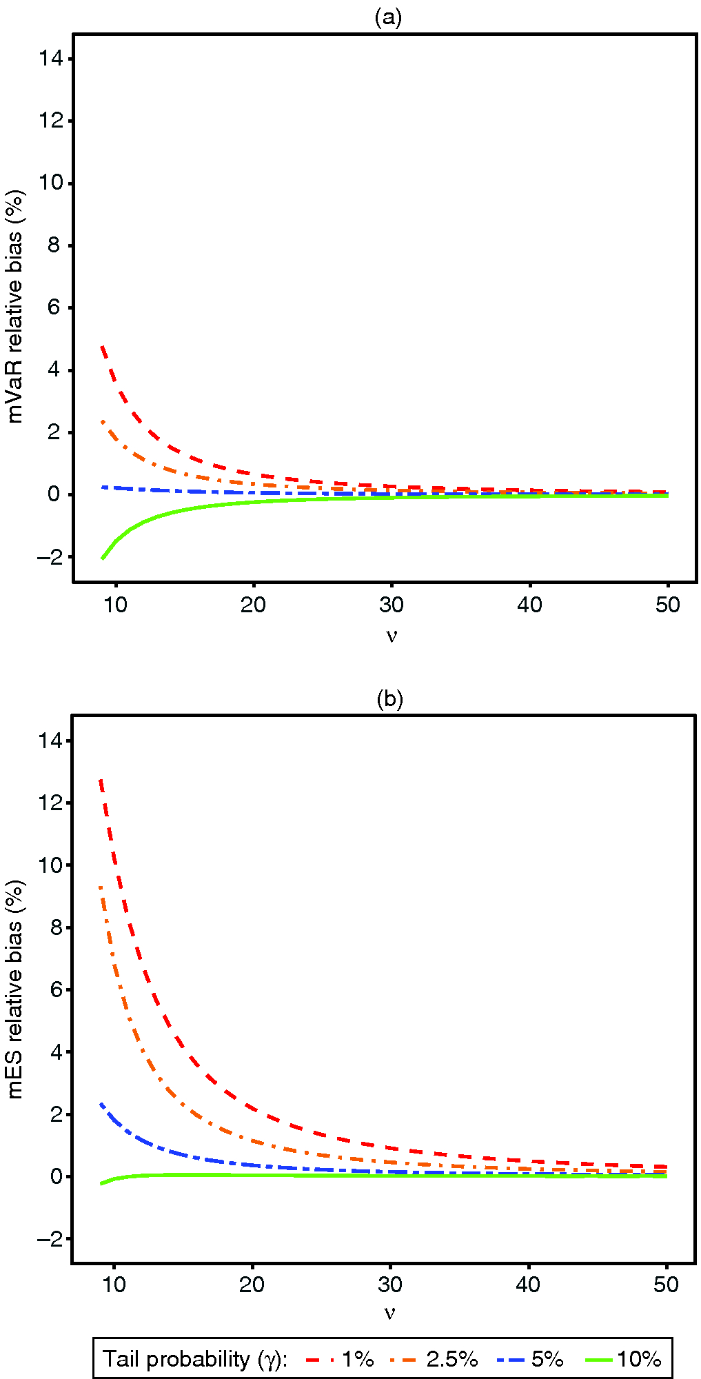
Figure 1: (a) mVaR and (b) mES asymptotic relative bias for $t$-distributions.

This decrease in bias toward zero with increasing degrees of freedom is quite evident in Figure 1(a) for all three tail probabilities. Note that the size of the relative bias is very sensitive to the tail probability through the quantile $z_{\gamma }$ for the mVaR estimator, and through the quantile $g_{\gamma }$ for the mES estimator. This explains the increasing differences between the relative bias curves for the three tail probabilities, as well as the larger relative biases of the mES estimator compared with those of the mVaR estimator, as $\nu$ approaches its smallest value in the plot (ie, 9).

3.4.1 Bias of normal distribution VaR and ES for $t$-distributions

In some contexts we might be tempted to use the normal distribution VaR MLE (nVaR) or normal distribution ES MLE (nES). For example, as pointed out by a referee, skewness or kurtosis in daily returns would be “averaged out” in cumulative returns for a ten-day period, and there would be no need for the modified estimators. However, a word of caution is in order concerning use of nVaR or nES based on the assumption of normality: if this assumption is wrong it can result in large-sample bias, for example, when the returns actually have a $t$-distribution. It is straightforward to check that the expressions for the asymptotic relative biases of nVaR and nES at standard $t$-distributions are given by

	${\mathrm{RB}}_{\text{nVaR},t\text{-dist}}$	$={\displaystyle \frac{1}{z_{\gamma }}}\left(\sqrt{{\displaystyle \frac{\nu -2}{\nu }}}{q}_{\nu ,\gamma }\right)-1,$		(3.19)
	${\mathrm{RB}}_{\text{nES},t\text{-dist}}$	$={\displaystyle \frac{1}{\varphi (z_{\gamma })}}\left(t_{\nu -2}\left(\sqrt{{\displaystyle \frac{\nu -2}{\nu }}}{q}_{\nu ,\gamma }\right)\right)-1.$		(3.20)

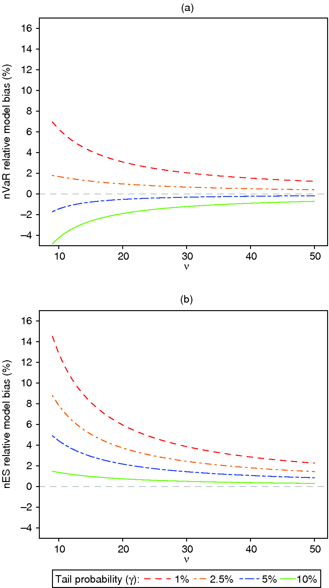
Figure 2: Normal distribution (a) nVaR and (b) nES asymptotic relative bias for t -distributions.

Figure 2 plots the asymptotic relative biases of nVaR and nES against the degrees of freedom $\nu$ for several values of $\gamma$. These biases tend to be larger than those of the mVaR and mES for the $t$-distributions in Figure 1. Further, the variances of nVaR and nES can be quite large at $t$-distributions. Thus it is unwise to use nVaR and nES unless careful statistical testing and/or model selection has led to such a choice. 

4 Efficiency and bias performance of modified value-at-risk and modified expected shortfall

In this section, we investigate the finite-sample RMSE efficiency and bias of mVaR and mES estimators relative to the MLEs for normal and $t$-distributions. One reason for the risk manager to be concerned about modified estimator efficiencies is that when a risk estimator has a low RMSE efficiency relative to that of the MLE, the MLE will be preferred to the modified estimator.

With $b_n$ the bias and ${\sigma }_n^2$ the variance of the estimator ${\widehat{\rho }}_n$, we define the RMSE efficiency of a modified estimator as the square root of the ratio of mean square errors:

$${\mathrm{EFF}}_n=\sqrt{\frac{{\mathrm{MSE}}_n({\widehat{\rho }}_{\mathrm{MLE},n})}{{\mathrm{MSE}}_n({\widehat{\rho }}_{\mathrm{mod},n})}}=\sqrt{\frac{b_{\mathrm{MLE},n}^2+{\sigma }_{\mathrm{MLE},n}^2}{b_{\mathrm{mod},n}^2+{\sigma }_{\mathrm{mod},n}^2}}.$$

(4.1)

The subscript $n$ in the estimator indicates its dependency on sample size. We compute finite-sample efficiency estimates

$${\widehat{\mathrm{EFF}}}_n=\sqrt{\frac{{\widehat{b}}_{\mathrm{MLE},n}^2+{\widehat{\sigma }}_{\mathrm{MLE},n}^2}{{\widehat{b}}_{\mathrm{mod},n}^2+{\widehat{\sigma }}_{\mathrm{mod}}^2}}$$

(4.2)

using the following Monte Carlo estimates of finite-sample bias and variance. For $M$ sets of sample returns of size $n$ from a standard normal or a standard $t$-distribution, we compute the relative bias estimates as

	${\widehat{\mathrm{RB}}}_{\mathrm{MLE}n}$	$={\displaystyle \frac{1}{\rho }}\left({\displaystyle \frac{1}{M}}{\displaystyle \sum _{m=1}^M}{\widehat{\rho }}_{\mathrm{MLE}n,m}\right)-1,$		(4.3)
	${\widehat{\mathrm{RB}}}_{\mathrm{mod}n}$	$={\displaystyle \frac{1}{\rho }}\left({\displaystyle \frac{1}{M}}{\displaystyle \sum _{m=1}^M}{\widehat{\rho }}_{\mathrm{mod}n,m}\right)-1,$		(4.4)

with the risk measure replicates ${\widehat{\rho }}_{\mathrm{MLE}n,m}$ and ${\widehat{\rho }}_{\mathrm{mod}n,m}$. Here, $\rho$ is the corresponding true risk measure value as defined in Table 1. The Monte Carlo variance estimates are just the sample variances of the $M$ risk measure estimates.

When relative biases are negligibly small the practitioner can compute finite-sample standard errors (SEs) from an asymptotic standard deviation formula by plugging in estimates of the unknown parameters and dividing the result by the square root of the sample size. These “projected SEs” can then be used to construct confidence intervals for mVaR and mES estimators in the usual manner using a normal distribution approximation. The finite-sample-size Monte Carlo results in this section provide guidance on whether relative biases are sufficiently small that such confidence intervals will be useful.

An additional consideration is how well the projected SEs approximate the true finite-sample SEs; our finite-sample studies below address this issue.

4.1 mVaR and mES estimator efficiencies and biases for normal distributions

We check the possibility of poor performance of mVaR and mES estimators for normally distributed returns by comparing their asymptotic standard error efficiencies, and by comparing their finite-sample and RMSE efficiencies and relative biases across tail probabilities ranging from 1% to 10%.

4.1.1 Modified estimators’ asymptotic efficiencies

For normal distributions, the mVaR and mES estimators are consistent estimators of the true VaR and ES, ie, they have zero asymptotic bias. The same is of course true of the VaR and ES maximum likelihood estimators. In this special case, it makes sense to analyze the asymptotic standard-error efficiency of mVaR and mES relative to the VaR and ES maximum likelihood estimators, respectively. These efficiencies are asymptotic versions of (4.1) with the bias terms set to zero, and the variances are the asymptotic variances. We have the asymptotic variance of the modified estimators from Section 3, and the asymptotic variance expressions for the VaR and ES maximum likelihood estimators for normal distributions are provided in the online appendix. The resulting asymptotic efficiencies are shown by the solid green line in Figure 3.

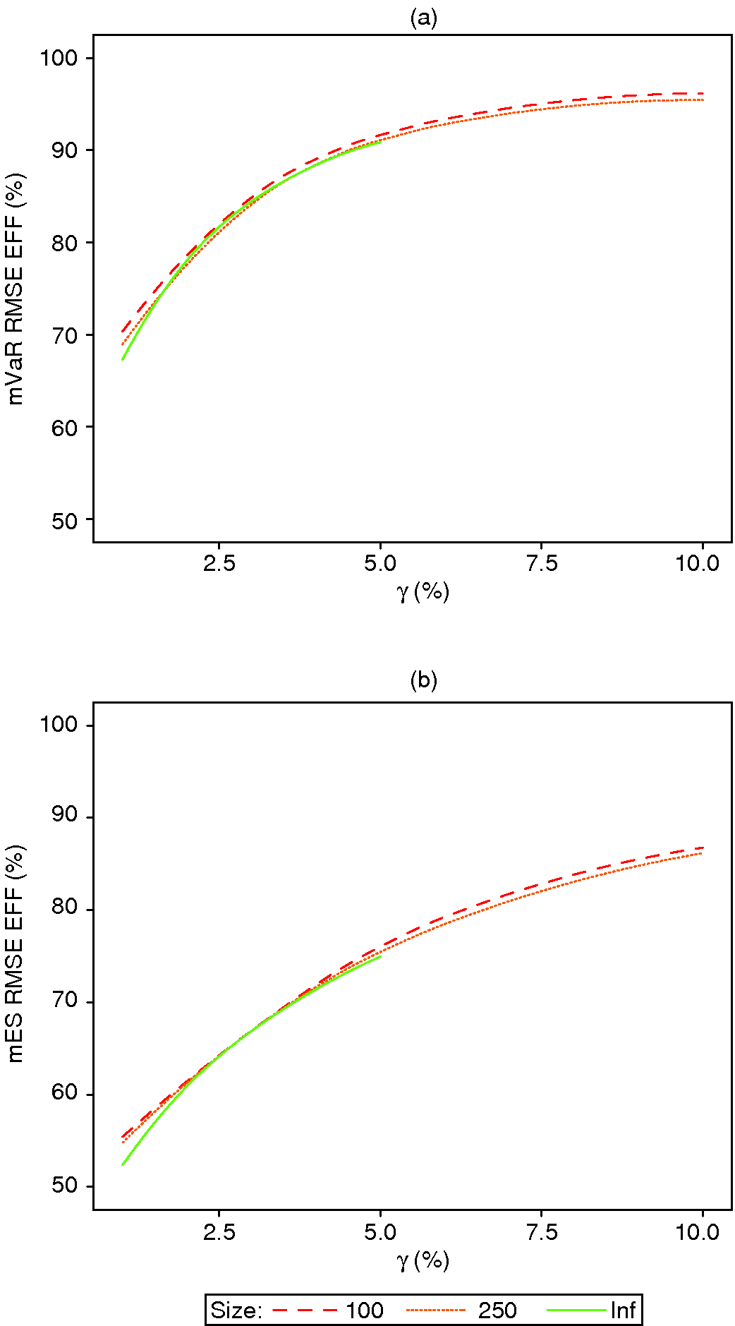
Figure 3: mVaR and mES efficiencies for normal distributions.

4.1.2 Modified estimators’ finite-sample RMSE efficiencies

Figure 3 displays the mVaR and mES finite-sample RMSE efficiencies for sample sizes 100 and 250 as dashed and dotted lines, respectively. Several points are immediately clear.

1. (1)

   For the normal distribution, the mVaR and mES finite-sample RMSE efficiencies in Figure 3 are extremely close to the asymptotic standard error efficiencies obtained by setting the biases equal to zero and using the asymptotic variances in (4.1), even for the relatively small sample size of 100. Thus, for normal distributions the asymptotic standard-error efficiencies provide an excellent proxy for the finite-sample RMSE efficiencies.

2. (2)

   For both mVaR and mES, we obtain higher efficiencies at higher tail probabilities, which from an efficiency point of view speaks in favor of using a 5% or 10% tail probability.

3. (3)

   Use of mES results in lower RMSE efficiency than use of mVaR.

4.1.3 Modified estimators’ finite-sample biases

Although the modified estimators have zero asymptotic bias for a normal distribution, they have nonzero finite-sample biases. We evaluate this finite-sample bias via Monte Carlo simulation using the relative bias estimator given by (4.4) and display the results for mVaR and mES in Figure 4.

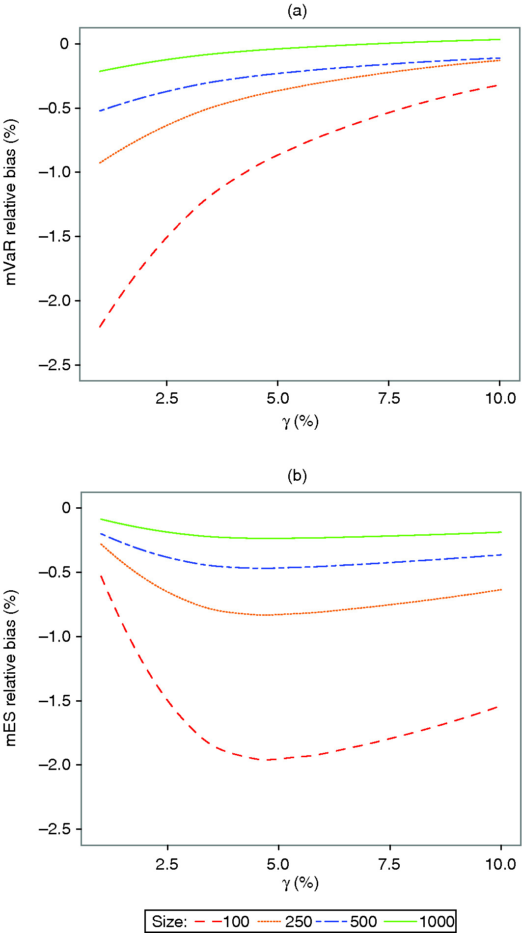
Figure 4: mVaR and mES finite-sample relative bias for normal distributions.

It is clear that the biases decrease toward zero with increasing sample size. At a sample size of $n=250$ and larger, the relative biases are less than 1.0% for both mVaR and mES, and for $n=500$ and larger the absolute biases are not more than 0.5%. For comparison, our calculations show that the finite-sample relative biases of the normal distribution VaR and ES MLE are very much smaller than those of the modified estimators in Figure 4.

A curious feature of the comparative finite-sample bias behavior of the mVaR estimator versus the mES estimator for a normal distribution is that, while the worst-case relative biases for the mVaR estimator occur at the smallest tail probability, those of the mES estimator occur at the largest tail probability. This is evidently due to the complicated small-sample behavior of the polynomials associated with the skewness and kurtosis estimators involved in the complex mES expression (3.4).

In summary, since a sample size of 250 or larger results in relative biases of less than 1% in absolute value, it seems quite safe to use projected SEs not only for their own sake, but also to construct confidence intervals, with the location of the confidence interval not being relatively biased by more than 1%.

4.1.4 Modified estimators’ projected standard errors

One remaining question is how well the projected SEs represent the true finite-sample SEs. The results in Figure 5 answer this question. For a tail probability of 2.5% mVaR the projected SEs underestimate the true SEs by 5% at a sample size of 250, and by less than 5% for larger sample sizes and larger tail probabilities. The situation is worse for mES at a sample size of 250 and 2.5% tail probability, where finite-sample SEs are underestimated by almost 10%; these are not much better at 5% tail probability. However, a reasonable way to improve finite-sample SEs and associated confidence intervals for the modified estimators would be to inflate the projected SEs by an appropriate amount, revealed in the figures, eg, by 5% for VaR and 10% for mES in the examples just cited.

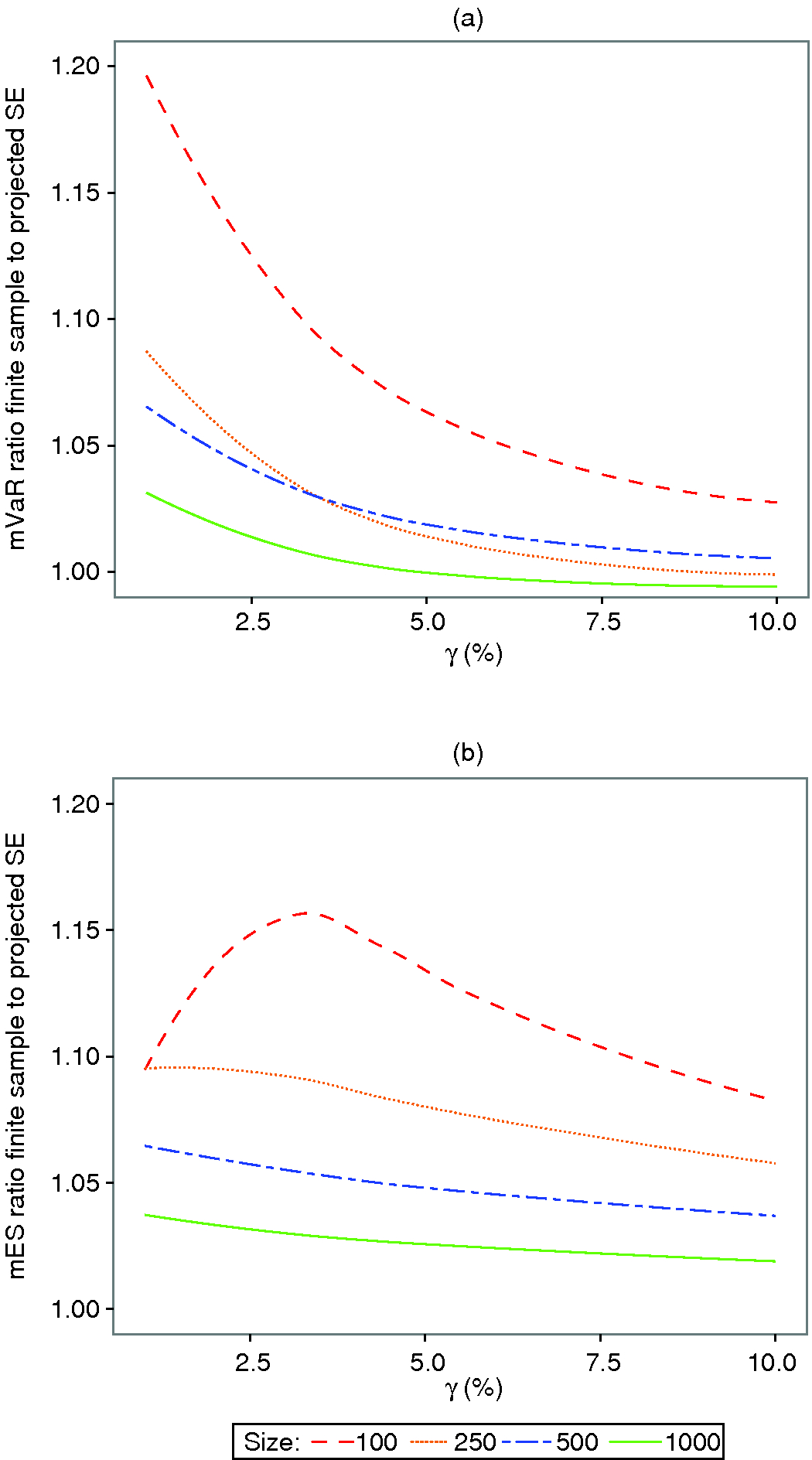
Figure 5: mVaR and mES finite-sample to projected SE ratios for normal distributions.

4.2 mVaR and mES RMSE efficiencies and biases for $t$-distributions

We now present the modified estimators’ finite-sample RMSE efficiencies and biases in the same manner as for the normal distribution results in the previous subsection. The main difference is that for a $t$-distribution the modified estimators have nonzero asymptotic bias.

  4.2.1 mVaR and mES finite-sample RMSE efficiencies for $t$-distributions  

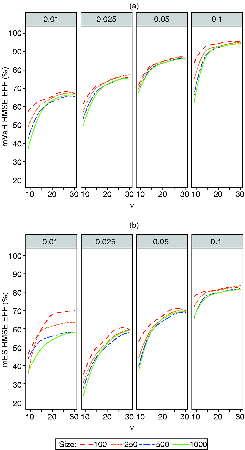
    Figure 6: (a) mVaR and (b) mES finite-sample RMSE efficiency for $t$-distributions.

    The pair of four-panel plots in Figure 6 display the RMSE efficiencies for mVaR and mES for $t$-distributions with unknown degrees of freedom ranging from 9 to 30. Except for the somewhat anomalous mES behavior at 1% tail probability, the general behavior of the efficiencies is similar to that for the normal distribution, in that efficiencies increase with increasing tail probability, with the best modified estimator performance being at 10% tail probability.²²Boudt et al (2008) discussed the unreliability of mES for small tail probabilities, and recommended a correction that ensures that mES is always at least as large as mVaR. In addition, mVaR efficiencies are higher than mES efficiencies, and increase slightly with decreasing sample size. Also, reassuringly, we see that the mVaR efficiencies at thirty degrees of freedom are very close to those for the normal distribution mVaR in Figure 3(a). And, for mES, except for tail probability 1%, the efficiencies for thirty degrees of freedom are reasonably close to the normal distribution efficiencies in Figure 3(b).

Most importantly, we see that, for all four tail probabilities, the RMSE efficiencies of both mVaR and mES decrease substantially as the degrees of freedom decrease. For mES at 2.5% tail probability and nine degrees of freedom, the average efficiency across the four sample sizes is about 30%; compare this with the 60% efficiency at the nearly normal $t$-distribution with thirty degrees of freedom. Such low efficiencies may encourage practitioners to use the VaR and ES MLEs when a $t$-distribution is justified empirically.

4.2.2 mVaR and mES finite-sample biases for $t$-distributions

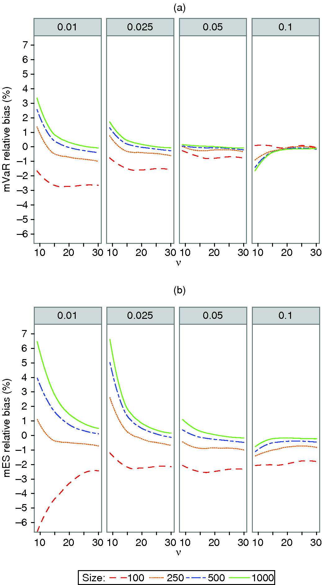
Figure 7: (a) mVaR and (b) mES finite-sample relative bias for $t$-distributions.

Figure 7 shows the finite-sample relative biases for the $t$-distribution. The behaviors of the relative biases with thirty degrees of freedom and all four tail probabilities are reasonably consistent with the normal distribution results in Figure 4. Note that the biases can take both negative and positive values, depending on the sample size and tail probability, except for the peculiar behavior of mVaR at 10% tail probability, where the relative biases increase from the most negative biases at a sample size of 100. With the exceptions of the modified estimators at 10% tail probability and mES at 1% tail probability, the relative biases increase with decreasing degrees of freedom.

In the case of mVaR at 2.5% tail probability and sample sizes 100, 250 and 500, there are small relative biases of not more than 1.5% in magnitude across all degrees of freedom considered. At 5% tail probability mVaR has even smaller absolute relative biases.

For mES with small degrees of freedom, the magnitudes of the relative biases across all sample sizes are much larger at tail probabilities 1% and 2.5%. However, if we use mES with tail probability 2.5% and a sample size of 250, the magnitude of the relative bias will be less than 3% for the entire range of degrees of freedom considered, which may be acceptable to a risk manager.

4.2.3 mVaR and mES projected standard errors for $t$-distributions

Ratios of projected SEs to true finite-sample SEs for the modified estimators for $t$-distributions with unknown degrees of freedom are shown in Figure 8. If we are willing to tolerate an mVaR underestimate as large as 20% in finite-sample SE across all degrees of freedom, then we can use a 2.5% tail probability and a sample size of 500 or larger; a sample size of 250 achieves almost the same result. But, if we are willing to use a 5% mVaR tail probability, then a sample of size 250 or larger will ensure an SE underestimate of not greater than 10%.

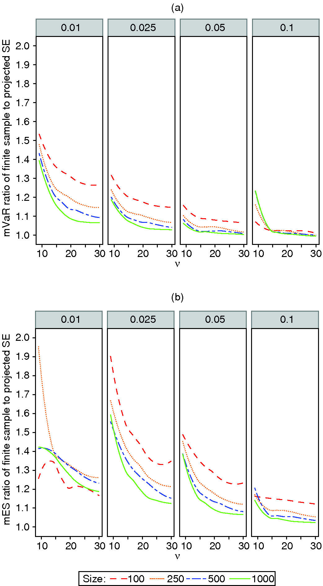
Figure 8: (a) mVaR and (b) mES finite-sample to projected SE ratios for $t$-distributions.

For mES at 2.5% tail probability, the projected SE underestimation is much worse, with a nine degrees of freedom underestimate of 90% at a sample size of 100 and of about 68% at a sample size of 250. One possibility would be to adjust the projected SE by an inflation factor to match the Monte Carlo estimate of the true finite-sample SE. The problem in doing so is the wide variability in the estimated finite-sample SE across different degrees of freedom. If we use an SE inflation factor to match the true finite-sample SE of nine degrees of freedom and the distribution turns out to be close to normal (say twenty to thirty degrees of freedom), then the confidence interval length may be grossly conservative. One simple approach could be to estimate degrees of freedom with a method-of-moments estimator and determine a projected SE inflation factor from the curves in Figure 8.

5 Concluding comments

We compared mVaR and mES estimators with VaR and ES under normal and fat tailed $t$-distributions by studying their asymptotic and finite-sample variance, bias and mean square error, and their statistical efficiency relative to maximum likelihood estimators of VaR and ES. We derived general expressions for the asymptotic variance of modified and MLE estimators of VaR and ES, and expressions for the asymptotic bias of the modified estimators. The MLEs are consistent estimators with zero asymptotic bias, and this is also the case for the modified estimators for normal distributions. However, the modified estimators have nonzero asymptotic biases for $t$-distributions that increase with both decreasing degrees of freedom and decreasing tail probability.

A key to the derivation of the large-sample variance of the mVaR and mES estimators was the asymptotic covariance matrix of the first four sample central moment estimators along with the multivariate delta method. A small but useful step in deriving the large-sample variance of the mES estimators was to translate the complex form of the estimator given by Boudt et al (2008) into a form very similar to the well-known form of mVaR estimators, ie, where coefficients of functions of skewness and kurtosis correction terms are polynomials in certain mVaR quantiles.

In addition to the asymptotic bias of the modified estimators for $t$-distributions, both modified estimators and MLEs have finite-sample biases. We analyzed the latter with finite-sample Monte Carlo studies of modified estimator performance at tail probabilities 1%, 2.5% (Basel III recommendation), 5% and 10%, and sample sizes 100, 250, 500 and 1000 with a focus on relative bias and RMSE efficiency.

For normal distributions, the key results are as follows:

1. (i)

   the finite-sample relative biases are sufficiently small to not be a problem for sample sizes of 250 and larger; and

2. (ii)

   the RMSE efficiencies are extremely well represented by the asymptotic standard deviation efficiencies at all sample sizes considered, with higher efficiencies for mVaR than mES, and increasing efficiency with increasing tail probability.

At the Basel III 2.5% tail probability, the mVaR normal distribution efficiency is 83%, while that of mES is about 64%. We believe that both may be considered tolerable by many risk managers.

For $t$-distributions the performance of mVaR and mES varies considerably across tail probabilities and sample sizes. Only some combinations of tail probabilities and sizes lead to biases that are sufficiently small such that the projected finite-sample standard errors obtained from the asymptotic variance formulas are both reliable indicators of estimator accuracy and useful for constructing bias-free confidence intervals. An mVaR estimator will have a negligibly small bias for $t$-distributions if used with 2.5% tail probability and a sample size of 250 or larger. A tail probability of 5% is preferable at a sample size of 100 or higher.

An mES estimator, on the other hand, will have tolerably small bias for $t$-distributions if used with a tail probability of 5% or 10% and a sample size of at least 250.

We focused on comparing the RMSE efficiency of mVaR and mES estimators with the corresponding VaR and ES MLEs. It may be natural to wonder how the modified estimators would perform against the nonparametric (“historical”) VaR and ES estimators (Martin and Zhang 2016). It remains to conduct a detailed evaluation of the performance of mVaR and mES relative to their nonparametric VaR and ES counterparts, keeping in mind that the comparison will be similar to that herein because of the bias of the modified estimators.

One limitation of our study in the context of independent and identically distributed returns is that we do not consider skewed fat-tailed distributions. We intend to complement the results of this paper with a sequel dealing with VaR and ES estimators for returns having skewed $t$-distributions, eg, the skewed $t$-distributions thoroughly studied by Azzalini and Capitanio (2003).

The performance of risk estimators in general in the presence of serial correlation in returns is an open problem for which there exists relatively little literature. Some initial work in this area has been done by Ledoit and Wolf (2008) for Sharpe ratio hypothesis testing with serial correlation, and by Chen (2008) for the asymptotic standard error of ES under serial correlation. This problem deserves more attention for risk measures in general, and for tail risk measures in particular.

Declaration of interest

R. Arora’s research for this paper was partly supported by funding from the Computational Finance and Risk Management Program in Applied Mathematics at the University of Washington. Computations were facilitated through the use of advanced computational, storage and networking infrastructure provided by the Hyak supercomputer system at the University of Washington, funded by the Student Technology Fee. The authors report no conflicts of interest. The authors alone are responsible for the content and writing of the paper.

Acknowledgements

The authors are thankful to the anonymous referees for their helpful suggestions in revising the manuscript.

References

Ardia, D., and Boudt, K. (2015). Testing equality of modified Sharpe ratios. Finance Research Letters 13, 97–104 (http://doi.org/f7dgkp).

Azzalini, A., and Capitanio, A. (2003). Distributions generated by perturbation of symmetry with emphasis on a multivariate skew $t$-distribution. Journal of the Royal Statistical Society B 65(2), 367–389 (http://doi.org/bndzz6).

Boudt, K., Peterson, B., and Croux, C. (2008). Estimation and decomposition of downside risk for portfolios with non-normal returns. The Journal of Risk 11(2), 79–103 (http://doi.org/b8h7).

Boudt, K., Carl, P., and Peterson, B. G. (2013). Asset allocation with conditional value-at-risk budgets. The Journal of Risk 15(3), 39–68 (http://doi.org/bwz4).

Chen, S. X. (2008). Nonparametric estimation of expected shortfall. Journal of Financial Econometrics 6(1), 87–107 (http://doi.org/frxvzq).

Ledoit, O., and Wolf, M. (2008). Robust performance hypothesis testing with the Sharpe ratio. Journal of Empirical Finance 15(5), 850–859 (http://doi.org/bjndtv).

Lehmann, E. L., and Casella, G. (1998). Theory of Point Estimation, 2nd edn. Springer Texts in Statistics, p. 590. Springer (http://doi.org/cmxmmh).

Maillard, D. (2012). A user’s guide to the Cornish Fisher expansion. Working Paper, Social Science Research Network (http://doi.org/b8h8).

Martin, D., and Zhang, S. (2016). Nonparametric versus parametric expected shortfall. Working Paper, Social Science Research Network (http://bit.ly/2rSVSY1).

Zangari, P. (1996). A VaR methodology for portfolios that include options. RiskMetrics Monitor 1(Q1), 4–12.

Download PDF Appendix 1

• Keywords
• Basel III
• Expected shortfall
• Value-at-risk (VAR)
• Original research
• More
  Less