Exploring the equity–bond relationship in a low-rate environment with unsupervised learning

Lucas Baynes; Giulio Renzi-Ricci

1 Introduction

Theory dictates that bond prices and interest rates are inversely related. In simple terms, when rates go up, prices go down. With the combination of low and rising interest rates, the principle implies that bond prices should fall. This raises the question: why include any fixed income exposure at all? Of course, simply considering this inverse relationship does not tell the whole story (see Renzi-Ricci and Baynes (2021) for further discussion).

Indeed, a whole host of financial literature reviews the valuable properties of bonds, with key conclusions from recent years highlighting that bonds are essential to achieve volatility reduction (Ryan 2021); that, unlike equities, they can perform well in low or negative growth environments (Podkaminer et al 2019); and that a sizable allocation to fixed income would have historically led to Sharpe ratio maximization (Gottesman and Morey 2021).

Another crucial property of bonds is that they act as a hedge against equity market drops. In these scenarios, there can be a flight-to-safety (Andersson et al 2008), where investors react by allocating more capital in safer investments such as government bonds, leading to a rise in their price. Moreover, equity market crashes themselves are often due to negative economic shocks, such as the Covid-19 pandemic (Papadamou et al 2021). Central banks typically respond to this by cutting rates and conducting quantitative easing, which usually results in a positive fixed income performance. For that reason, investment principles would suggest that bonds still have a role to play in a portfolio.

In this paper, we consider this property from a new viewpoint. Due to increased computer processing power, the popularity of applying machine learning (ML) techniques in finance has increased considerably, with applications such as accomplishing outperformance (López de Prado 2016), novel portfolio construction techniques (Aydemir 2020; Lim and Ong 2021) and dynamic replication and hedging (Kolm and Ritter 2019) helping to expand the knowledge frontier. However, such applications are often technical and can be difficult to interpret for advisors and clients whose expertise usually lies in other areas. Therefore, in this paper we look to bridge that gap and democratize an unsupervised learning technique called $k$ -means clustering by applying it to historical returns during periods of low government bond yields. This method – to the best of the authors’ knowledge, never before used in this context – brings new insight to the traditional analysis conducted on stock–bond diversification and allows us to intuitively identify the market states that govern the equity–bond relationship during low-rate periods. Our results suggest an enduring role for bonds as a hedge against equity risk even when yields are low.

2 The equity–bond relationship: the past two decades

Historically, the correlation between equities and bonds has changed from negative to positive on multiple occasions, but it has been predominately negative since the late 1990s.¹¹ 1 There are several studies focusing on the underlying drivers of the relationship and the correlation between equities and bonds, including Wainscott (1990), Ilmanen (2003), Yang et al (2009), Baele et al (2009) and Wu et al (2022). In this paper, we look at this well-studied topic from a new angle through the application of ML.

Also, compared with corporate bonds, government bonds tend to have a lower correlation with equities. Therefore, in this paper we focus on the relationship between equities and government bonds rather than aggregate bonds. In particular, we look at the monthly performance of equities and government bonds between October 2000 and March 2021 for US and global indexes. We also make it a condition that the government bond yield for these returns must be below a certain threshold, in order to isolate the relationships that have historically held when interest rates are low. As we will see, over this period there are cases in which both equities and bonds have had positive returns (ie, the pairwise returns lie in an “up–up” state), cases in which equities have had positive returns but bonds have had negative returns (“up–down”), and, conversely, there have been cases in which pairs of returns have been in the “down–up” and “down–down” states. From an investor’s perspective, an ideal world would be one in which returns only lie in the “up–up” state. However, this is rarely the case and what we are really concerned with is how bonds perform in states in which equities have shown negative performance.

One approach to assess this could be to simply count the observations that fall into each of the four different quadrants, giving a sense of how frequently each market state happens. For example, when US equities show negative performance in our data set, US government bonds show positive performance roughly 63% of the time. However, this tells us nothing about the magnitude; perhaps bonds show small positive performance most of the time but there are a few scenarios in which both equities and bonds drop significantly (the remaining 37%). If that were the case, it would be unreasonable to say that bonds are good hedges against poor equity performance – in times of turmoil the last thing an investor wants is for both of their asset classes to lose money.

An alternative approach might be to use regression techniques and to determine a line of best fit, giving us a sense of the bonds’ average response for a given change in equities. However, as we will show later in this paper, there are significant amounts of dispersion and noise that a linear regression model would not be able to capture. Moreover, a regression approach would be unable to provide any sense of whether certain scenarios (eg, both bonds and equities having negative returns) can be considered as actual market states that are likely to recur in the future, or are simply the result of market volatility and noise. Therefore, we require a methodology that addresses both issues. One way of doing this is to use $k$ -means clustering, in which we use ML to determine what the different clusters of pairwise returns are. This can give us a sense of which kinds of scenarios can be considered market states (and which cannot) and how bonds perform when equities fall. Therefore, our approach allows us to shed more light on the equity–bond relationship than any other techniques can, and it can be used as a complementary tool for investors.

3 Clustering analysis of equity–bond return pairs

3.1 US returns

One of the most widely used types of unsupervised ML is $k$ -means clustering. With this technique, $k$ represents a given number of clusters (decided by the user) and observations are categorized such that those that fall into the same cluster are the most like each other, while simultaneously being as dissimilar as possible to the observations in other clusters.²² 2 Goodfellow et al (2016) define unsupervised learning as any technique that determines information from a “distribution that (does) not require human labor to annotate examples”.

Note that, by applying unsupervised learning to our return pairs, we do not make any claims as to what type of returns they are. We simply run them through an unsupervised learning algorithm, which then tells us the type based on the return pairs’ similarities.

As mentioned above, in order to hone in on the low-rate environment, we only consider returns for which the government bond yield for that period is below a certain threshold.³³ 3 We also conducted this analysis for the entire period (ie, without the threshold) and it showed very similar results to those presented. Our yield threshold for the US is 2.5% (ie, for any given month, the US 10-year Treasury yield at the beginning of that month must be below 2.5% in order for the return pair for that month to feature in our analysis). This threshold was chosen to ensure that the analysis applies to a low-rate environment while including a reasonably large number of return pairs. In Figure 1 we show the results of the $k$ -means clustering algorithm run on these US returns when $k$ is equal to 2 or 3.⁴⁴ 4 The algorithm is not actually applied on the returns themselves but on their standardized $z$ -scores. We then map the clustered $z$ -scores back onto their return equivalents.

Plots of k-means clustering on US government bond returns and US equity returns for (a) k=2 and (b) k=3. Equity returns refer to the MSCI USA Total Return Index and bond returns refer to the Bloomberg US Treasury Total Return Index. The yield threshold of 2.5% was based on the US 10-year Treasury bond. All figures are in US dollars. Clusters' centroids are indicated by diamonds. Source: based on monthly Bloomberg L.P. data from October 2000 to March 2021. Past performance is no guarantee of future returns. The performance of an index is not an exact representation of any particular investment, as you cannot invest directly in an index. — Figure 1: Plots of $k$ -means clustering on US government bond returns and US equity returns for (a) $k=\text{2}$ and (b) $k=\text{3}$ . Equity returns refer to the MSCI USA Total Return Index and bond returns refer to the Bloomberg US Treasury Total Return Index. The yield threshold of 2.5% was based on the US 10-year Treasury bond. All figures are in US dollars. Clusters’ centroids are indicated by diamonds. Source: based on monthly Bloomberg L.P. data from October 2000 to March 2021. Past performance is no guarantee of future returns. The performance of an index is not an exact representation of any particular investment, as you cannot invest directly in an index.

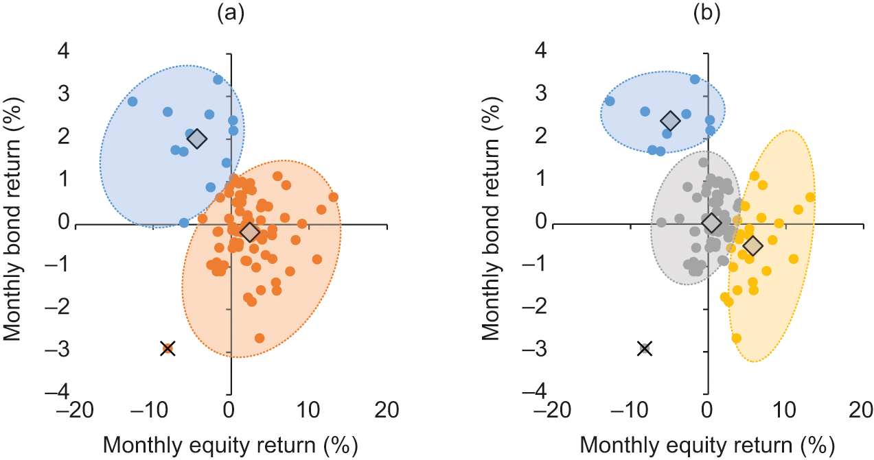
Each of the clusters is given a color. We observe that for $k=2$ , some returns are categorized as orange (in which equities have almost always had positive performance and bonds are slightly negatively tilted) and some as blue (in which bonds have almost always shown positive performance and equities have shown negative performance). In other words, this suggests a negative relationship between US equity and US Treasury returns and that when equities go up, the bond return is not easily predictable but, when equities go down, bonds almost always go up. Importantly, we do not see a cluster located in the “down–down” quadrant, implying that the few pairs of returns that do fall in this region are anomalous and not statistically relevant. For $k=3$ , the situation is very similar. The blue “down–up” state largely remains unchanged, while the orange “up–down” state splits into two distinct market states: gray and yellow. This reinforces the hypothesis that bonds provide good diversification for equities, as again we do not see a cluster toward the bottom-left corner mapping a “down–down” market state.

The diamonds depict each cluster’s centroid, which is not an actual return pair but rather the notional center of each cluster. For the example of $k=2$ , this categorization can be thought of as two market state centers: one that has equities up and bonds slightly down and one that has equities down and bonds up. For $k=3$ , we still have our state in which equities are down and bonds are up, and our “equities up” state now divides into two further states: one where bond returns are more centered on 0% and one where they are negative. This further confirms the idea that US Treasuries act as a counterbalance to equity movements.

To further corroborate the fact that the return pairs in the “down–down” quadrant are anomalous and not statistically relevant, we performed an anomaly detection analysis. Some papers (see, for example, Barai and Dey 2017) have used clustering techniques to perform anomaly detection, which helps to distinguish which observations may not be meaningful based on how far away they lie from their corresponding cluster centroid. We performed a version of this (see Appendix 1 online) to assess which observations may be anomalies, denoted in the figures by black crosses. We observe that, irrespective of whether $k=2$ or $k=3$ , there is a single anomaly that lies in the bottom-left quadrant. Intuitively, this suggests that scenarios in which equities and bonds have negative unidirectional returns are rare and can be considered anomalous, further corroborating the conclusion that bonds act as a good hedge for equities.

We also mentioned earlier that an alternative approach to this analysis might be to run a linear regression in order to gain a sense of the bonds’ average response for a given change in equities. However, a line of best fit through these data points would be unable to explain a large percentage of the variance (ie, it would have a low $R$ -squared value, in this case equal to 9.9%) due to the large dispersion of the return pairs. Therefore, while it might provide some indication as to the typical directionality of the relationship, it would not help much in understanding the different market states that our clustering analysis gives us. More detail on such an approach is provided in Appendix 2 (online).

At this stage, there are two questions: “Should we use $k=2$ or $3$ ?” and “Why should $k=2$ or $3$ ?” We used two well-established techniques to determine the appropriate number of clusters (see Appendix 3 online). Our results suggest that the use of two clusters is the best choice for the US data based on both validation methods.⁵⁵ 5 Some qualitative judgment is still required when choosing an appropriate value for the number of clusters – in this, parsimony is often best. In fact, it can be the case that some of the validation methods (eg, silhouette score) suggest multiple clusters to be optimal, which can lead to overfitting.

This result is important because it suggests that there are most likely no more than two main states that are consistent with the underlying pattern of equity and bond returns and that these two states (“up–down” and “down–up”) identified by the clusters correspond to US equities and government bonds balancing one another. Other return pairs are interpreted as not statistically significant deviations from these two main states. The fact that, when we increase the number of clusters to three, the “up–down” cluster is further split into two new clusters and the three centroids are aligned on an imaginary negatively sloped line confirms the diversification properties of government bonds.

A key advantage of this analysis over a regression-based approach is the identification of market states. In addition to providing information on the (linear) relationship between equities and bonds, $k$ -means clustering enables us to identify any clustering that may be consistent with the presence of a specific market state (eg, “down–up”). The combination of using the optimal number of clusters and their locations helps to assess whether there is sufficient evidence for such a state to exist. Moreover, with $k$ -means clustering, the absence of clusters can also provide valuable insight into whether observations located in these regions are likely to recur in the future.

3.2 Global returns

Of course, not all multi-asset investors choose to invest exclusively in US funds. For this reason, we also examine global returns to see whether this relationship holds for global investors. Figure 2 shows the same $k$ -means analysis when using $k$ equal to 2 or 4 for global returns. Here, we set our yield threshold equal to 1.5% using a global Treasury index that resulted in a similar number of return pairs as the US example.

Plot of k-means clustering on global government bond returns and global equity returns for (a) k=2 and (b) k=4. Equity returns refer to the MSCI All Country World Total Return Index and bond returns refer to the Bloomberg Global Treasury Total Return Index. The yield threshold of 1.5% was based on the Bloomberg Global Treasury Total Return Index. All figures are in US dollars and bond returns are hedged to US dollars. Clusters' centroids are indicated by diamonds. Source: based on monthly Bloomberg L.P. data from October 2000 to March 2021. Past performance is no guarantee of future returns. The performance of an index is not an exact representation of any particular investment, as you cannot invest directly in an index. — Figure 2: Plot of $k$ -means clustering on global government bond returns and global equity returns for (a) $k=\text{2}$ and (b) $k=\text{4}$ . Equity returns refer to the MSCI All Country World Total Return Index and bond returns refer to the Bloomberg Global Treasury Total Return Index. The yield threshold of 1.5% was based on the Bloomberg Global Treasury Total Return Index. All figures are in US dollars and bond returns are hedged to US dollars. Clusters’ centroids are indicated by diamonds. Source: based on monthly Bloomberg L.P. data from October 2000 to March 2021. Past performance is no guarantee of future returns. The performance of an index is not an exact representation of any particular investment, as you cannot invest directly in an index.

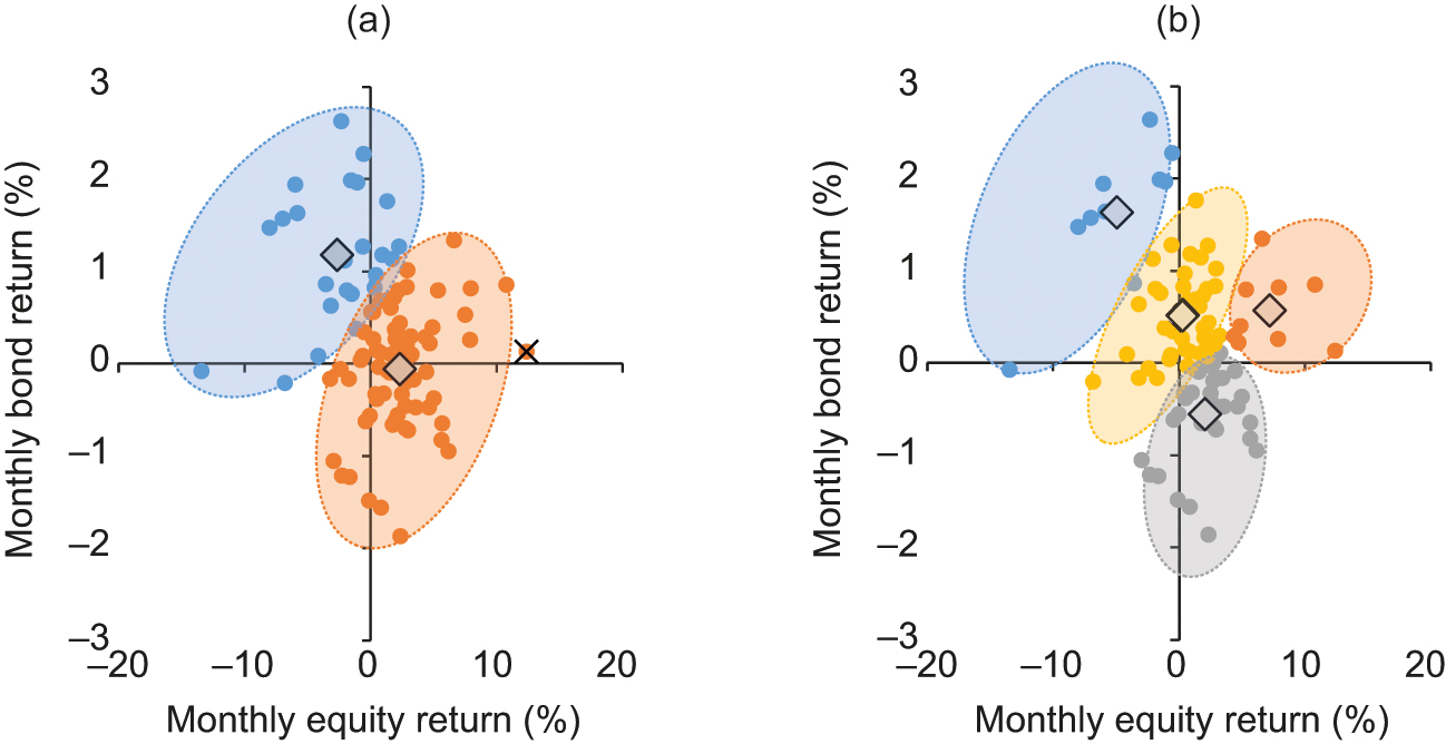
We see similar results as those in Figure 1, in the sense that two clusters show a clear diversification benefit with similar locations for the two centroids and, as a regression analysis would suggest, express a negative relationship between global equity returns and government bond returns. Again, there is no mapping to the “down–down” state, although one key difference from the US analysis is that an anomaly is detected in the top-right quadrant when $k=2$ , again suggesting that such unidirectional returns are rare. Therefore, at least in the paradigm of two clusters being appropriate, there seems to be little difference between US and global returns, with both characterizing recurrent market states as “equities up/bonds down” and “equities down/bonds up”.

Another difference between the global analysis and the US one is demonstrated in Figure A-4 (see the online appendix). Although it suggests that setting $k=2$ is still best when both the maximum silhouette score and the elbow occur at this point, in this case we see that $k=3$ has a lower silhouette score than $k=4$ , which is why we present our clustering with $k=4$ . However, there is still no cluster or centroid that lies in the bottom-left quadrant. Also, for $k=4$ , no anomalies were detected.

4 Conclusion

Investors have become concerned about the low-interest-rate environment due to the expected returns for fixed income. However, by conducting an analysis with an unsupervised ML technique called $k$ -means clustering, we show that government bonds have historically acted as a counterbalance in equity–bond portfolios during low-rate periods by hedging against equity market drops for both US and global investors. Although there are some months in which both equities and bonds fall, our analysis suggests that these can be thought of as market noise and distinct from the typical outcomes, which can be best thought of as recurrent “equities up/bonds down” and “equities down/bonds up” market states.

Declaration of interest

The authors report no conflicts of interest. The authors alone are responsible for the content and writing of the paper.

Note on risks

All investing is subject to risk, including the possible loss of the money you invest. Be aware that fluctuations in the financial markets and other factors may cause declines in the value of your account. There is no guarantee that any particular asset allocation or mix of funds will meet your investment objectives or provide you with a given level of income. Diversification does not ensure a profit or protect against a loss. Bonds are subject to interest rate risk, which is the chance bond prices overall will decline because of rising interest rates, and credit risk, which is the chance a bond issuer will fail to pay interest and principal in a timely manner or that negative perceptions of the issuerâs ability to make such payments will cause the price of that bond to decline. Investments in stocks and bonds issued by non-US companies and foreign governments are subject to risks including country/regional risk and currency risk. These risks are especially high in emerging markets.

References

Andersson, M., Krylova, E., and Vähämaa, S. (2008). Why does the correlation between stock and bond returns vary over time? Applied Financial Economics 18(2), 139–151 (https://doi.org/10.1080/09603100601057854).
Aydemir, Z. (2020). Portfolio construction using first principles preference theory and machine learning. Journal of Financial Data Science 2(4), 105–123 (https://doi.org/10.3905/jfds.2020.2.4.105).
Baele, L., Bekaert, G., and Inghelbrecht, K. (2009). The determinants of stock and bond return comovements. Review of Financial Studies 23(6), 2374–2428 (https://doi.org/10.1093/rfs/hhq014).
Barai, A., and Dey, L. (2017). Outlier detection and removal algorithm in $k$ -means and hierarchical clustering. World Journal of Computer Application and Technology 5(2), 24–29 (https://doi.org/10.13189/wjcat.2017.050202).
Goodfellow, I., Bengio, Y., and Courville, A. (2016). Deep Learning. MIT Press, Cambridge, MA.
Gottesman, A., and Morey, M. (2021). The argument for bonds in strategic asset allocation. Journal of Wealth Management 24(3), 43–57 (https://doi.org/10.3905/jwm.2021.1.150).
Iglewicz, B., and Hoaglin, D. (1993). How to Detect and Handle Outliers. ASQC Basic References in Quality Control: Statistical Techniques, Volume 16. ASQC Quality Press, Milwaukee, WI.
Ilmanen, A. (2003). Stock–bond correlations. Journal of Fixed Income 13(2), 55–66 (https://doi.org/10.3905/jfi.2003.319353).
Kolm, P., and Ritter, G. (2019). Dynamic replication and hedging: a reinforcement learning approach. Journal of Financial Data Science 1(1), 159–171 (https://doi.org/10.3905/jfds.2019.1.1.159).
Lim, T., and Ong, C. (2021). Portfolio diversification using shape-based clustering. Journal of Financial Data Science 3(1), 111–126 (https://doi.org/10.3905/jfds.2020.1.054).
López de Prado, M. (2016). Building diversified portfolios that outperform out of sample. Journal of Portfolio Management 42(4), 59–69 (https://doi.org/10.3905/jpm.2016.42.4.059).
Papadamou, S., Fassas, A., Kenourgios, D., and Dimitriou, D. (2021). Flight-to-quality between global stock and bond markets in the COVID era. Finance Research Letters 38, Paper 101852 (https://doi.org/10.1016/j.frl.2020.101852).
Podkaminer, E., Tollette, W., and Siegel, L. (2019). Preparing a multi-asset class portfolio for shocks to economic growth. Journal of Portfolio Management 45(2), 106–116 (https://doi.org/10.3905/jpm.2018.45.2.106).
Renzi-Ricci, G., and Baynes, L. (2021). Hedging Equity Downside Risk with Bonds in the Low-Yield Environment. Vanguard Group, Valley Forge, PA.
Ryan, L. (2021). Bonds don’t need to be negatively correlated with equities. Journal of Investing 30(6), 70–80 (https://doi.org/10.3905/joi.2021.1.192).
Wainscott, C. (1990). The stock–bond correlation and its implications for asset allocation. Financial Analysts Journal 46(4), 55–60 (https://doi.org/10.2469/faj.v46.n4.55).
Wu, B., Yeo, B., DiCiurcio, K., and Wang, Q. (2022). Forecasting US equity and bond correlation: a machine learning approach. Journal of Financial Data Science 4(1), 76–86 (https://doi.org/10.3905/jfds.2022.4.1.076).
Yang, J., Zhou, Y., and Wang, Z. (2009). The stock–bond correlation and macroeconomics conditions: one and a half centuries of evidence. Journal of Banking and Finance 33(4), 670–680 (https://doi.org/10.1016/j.jbankfin.2008.11.010).