Neural network middle-term probabilistic forecasting of daily power consumption

Roberto Baviera and Michele Azzone

Abstract

Middle-term horizon (months to a year) power consumption prediction is a major challenge in the energy sector, particularly when probabilistic forecasting is considered. We propose a new modeling approach that incorporates trend, seasonality and weather conditions as explicative variables in a shallow neural network with an autoregressive feature. Applying it to the daily power consumption in New England, we obtain excellent results for the density forecast on the one-year test set. We verified the quality of the power consumption probabilistic forecasting achieved not only by comparing the results with other standard models for density forecasting but also by considering measures that are frequently used in the energy sector, such as the pinball loss function and confidence interval backtesting.

Download PDF

Introduction

1 Introduction

Power consumption forecasting is crucial in the energy sector. In particular, middle-term forecasting, ie, on a time horizon of between a few months and a year,¹¹ 1 As standard in the literature, we refer to short-term consumption forecasting as the prediction of the consumption over an interval ranging from minutes to a few weeks, and to long-term consumption forecasting as the prediction for time horizons of over one year. plays a key role in the planning of power systems both for future generation plants and for transmission grids (see, for example, Hong and Fan 2016). Further, a reliable power consumption forecast also has consequences for network reliability and leads to a reduction in energy costs and carbon emissions.

Utilities and grid operators prefer to obtain a probabilistic forecast of the power consumption rather than a point forecast. A probabilistic forecast not only provides the future expected value but also informs us about the expected distribution. This technique gained momentum in the energy sector after the 2014 Global Energy Forecasting competition (GEFCom) on a power data set of New England in the United States (see, for example, Hong and Fan (2016), Nowotarski and Weron (2018) and the references therein). This competition was followed by another GEFCom in 2017, which awarded the best hierarchical forecasting and probabilistic forecasting model. Both competitions attracted participants from industry and academia. In this study, we focus on the 2017 GEFCom data set.

The key issue in model selection is to identify the correct features of the problem and their relationship with power consumption; this allows us to understand and hedge the risks that arise from unexpected jumps in consumption. We are interested in the impact of weather conditions on power consumption; these play a more relevant role in middle-term forecasts than economic and demographic drivers, which play a role in longer forecasts (see, for example, Hyndman and Fan 2010). We aim to model the dependency on weather conditions over the middle term; the most natural technique, now standard in power consumption forecasting, is known as ex post forecasting. It has been applied to middle-term probabilistic forecasting of power consumption on the French distribution network (Goude et al 2013) and on the Australian National Electricity Market (Hyndman and Fan 2010).

We use a machine learning technique. These techniques have been shown to provide interesting results in short-term point consumption forecasts (see, for example, Fan and Chen 2006; Meng et al 2009; Shi et al 2018). In this paper, we consider a neural network (NN). Most commonly, an NN returns the expected value, ie, a single-point forecast, for each time step and is therefore referred to as a point-forecasting method. As already mentioned, market players consider more interesting probabilistic forecasting methods that provide information on the distribution of future values. However, the literature on probabilistic forecasting of electrical consumption via NNs is quite recent and rather limited. This technique has been considered only by Vossen et al (2018) for one-hour density forecasting at the household level. The idea is to have the vector of parameters of the density as the NN output instead of the single-point forecast, and to maximize the logarithm of the likelihood. This idea was introduced for financial time series by Ormoneit and Neuneier (1996), but since then it has seldom been considered in the financial and energy literature (see, for example, Felder et al 2010; Nikolaev et al 2013). We consider the simple case of a Gaussian density forecast, following the results achieved in Baviera and Messuti (2020) using Gaussian processes for density forecasting of power consumption of one operator in North East England. These results for Gaussian density forecasts look promising in terms of both sharpness and reliability.

In this study, we apply an NN to density forecasting for middle-term consumption of up to one year: this is the first difference from Vossen et al (2018), who focus on short-term forecasting. Moreover, the main successes of NNs have been obtained on big data sets, where this technique is reliable and efficient (see, for example, LeCun et al (2015) and the references therein). The real challenge is to use these techniques with small data sets. This is a common demand in this industrial sector due to the rapid changes observed in the electricity market. To show the effectiveness and the quality of the proposed technique, we consider an extreme case, where we train our model on a few years’ data sets and predict daily power consumption on a one-year horizon. To the best of our knowledge, the use of NNs for middle-term density forecasting is new to the literature.

In this way, we can compute the densities of the consumption forecast for the proposed hybrid model, obtaining much better performance than with standard benchmark models, such as the ARX (see, for example, Box et al 2015, pp. 534ff) and other machine learning approaches, such as the Gaussian process (see, for example, Rasmussen and Williams 2006). The models’ performance is evaluated by comparing the forecasted results and the realized consumption on a one-year test set. To value the quality of the forecasting, we consider techniques that are standard either in the energy sector, such as the pinball loss function (see, for example, Nowotarski and Weron 2018), or in the banking sector after the introduction of Basel II, such as backtesting (Kupiec 1995; Christoffersen 1998).

The main contributions of this paper are threefold. First, we introduce a hybrid model that combines the advantages of classical univariate time series analysis and a shallow NN. In particular, we incorporate the dependency on weather conditions and previous times into the power consumption density forecast via an NN: the network structure we propose is new to the literature and is designed to yield both density forecasts and the autoregressive feature observed in the time series. Second, we show that an NN technique relying on a small data set (with only a few year-long training windows) achieves an excellent middle-term forecast of power consumption using only weather data. Third, we value the density forecasting via some sharpness and reliability measures, showing the quality of the results achieved. In particular, we show, with a method designed for machine learning techniques, that our results are not only accurate but also robust over time.

The rest of the paper is organized as follows. In Section 2, we summarize the key characteristics of the data set we analyze. In Section 3, we present the methodology; in particular, we describe in detail the proposed model and how the weather conditions are introduced in the NN as well as the forecasting technique and the evaluation methods. Sections 4 and 5 show the main numerical results, and Section 6 states our conclusions.

2 Description of the data set

New England is a region composed of six states in the northeastern United States. In 2010, New England accounted for approximately 5% of the US population. We use the 2017 GEFCom data set on household consumption in New England. This contains the data published by the overseer of the New England bulk electric power system, ISO New England (ISONE). The ISONE load data (on households’ consumption) includes the aggregated consumption of the whole New England area and eight different New England zones: each state corresponds to a zone, with the exception of Massachusetts, which is composed of three zones. The data set is available via the ISONE zonal information page and is updated periodically. At the time of 2017 GEFCom, the data set included data up to March 2017.²² 2 More than 300 academic and industry professionals, divided into 177 teams, participated in 2017 GEFCom. The competition featured two different tracks: the open-data track and the defined-data track. We use the data set of the defined-data track. The load data contains aggregated hourly household consumption in megawatt hours (MWh) together with averaged wet- and dry-bulb hourly temperatures in Fahrenheit (${}^{\circ }$F).³³ 3 The temperature in Celsius (${}^{\circ }$C) is equal to the temperature in Fahrenheit (${}^{\circ }$F) minus 32, times 5/9. We work with daily data for the whole New England area.

We aggregate the power consumption values and average the weather conditions, ie, we consider the daily consumption and the average temperature for every day. The weather data set represents the daily average of hourly records of weather conditions for the whole New England region. It includes two different variables: dry-bulb temperature in ${}^{\circ }$F and wet-bulb temperature in ${}^{\circ }$F.

We select 10 calendar years of the 2017 GEFCom data set, from January 2007 up to December 2016. We use the year 2011 to validate the calibrated model and select the best hyperparameters, the year 2012 for testing and the years 2013–16 to verify the robustness and reliability of the results achieved with the selected model. The years from 2007 to 2010 are used for calibration. The time line in Figure 1 describes the data segmentation.

Figure 1: The time line describes the data segmentation that we use to calibrate, validate, test and check the robustness of the proposed model. We calibrate the model on the years before 2011 and select the best model hyperparameters on the validation set (2011). We test the performance of the model on 2012 and check its robustness on the years 2013–16.

Table 1 gives descriptive statistics about daily power consumption and weather data on the 2007–10 time window. We remove February 29 to preserve the seasonality structure in leap years.

Table 1: Descriptive statistics for cumulative daily power consumption and average daily weather data in New England for the 2007–10 time window.

					Standard
	Min	Max	Mean	Median	deviation
Consumption (GWh)	$-$270.29	520.28	353.08	346.20	41.09
Dry-bulb temperature (${}^{\circ }$F)	00$-$4.80	085.83	049.66	050.94	17.73
Wet-bulb temperature (${}^{\circ }$F)	0$-$13.04	072.46	037.80	038.56	18.91

The yearly and weekly seasonality of power consumption is noticeable in the data set. In Figure 2, we plot two years (2009 and 2010) of electricity consumption. We infer a yearly seasonal behavior with two peaks per year (winter and summer). The peak in summer is due to air-conditioning, while the one in winter is due to heating.

Figure 2: Cumulated power consumption in New England (solid red line) between January 2009 and December 2010 with the fitted seasonal behavior (dashed green line). We can notice a yearly seasonal behavior (with two peaks per year in summer and winter) and locally lower values on Sundays (marked with the blue circles).

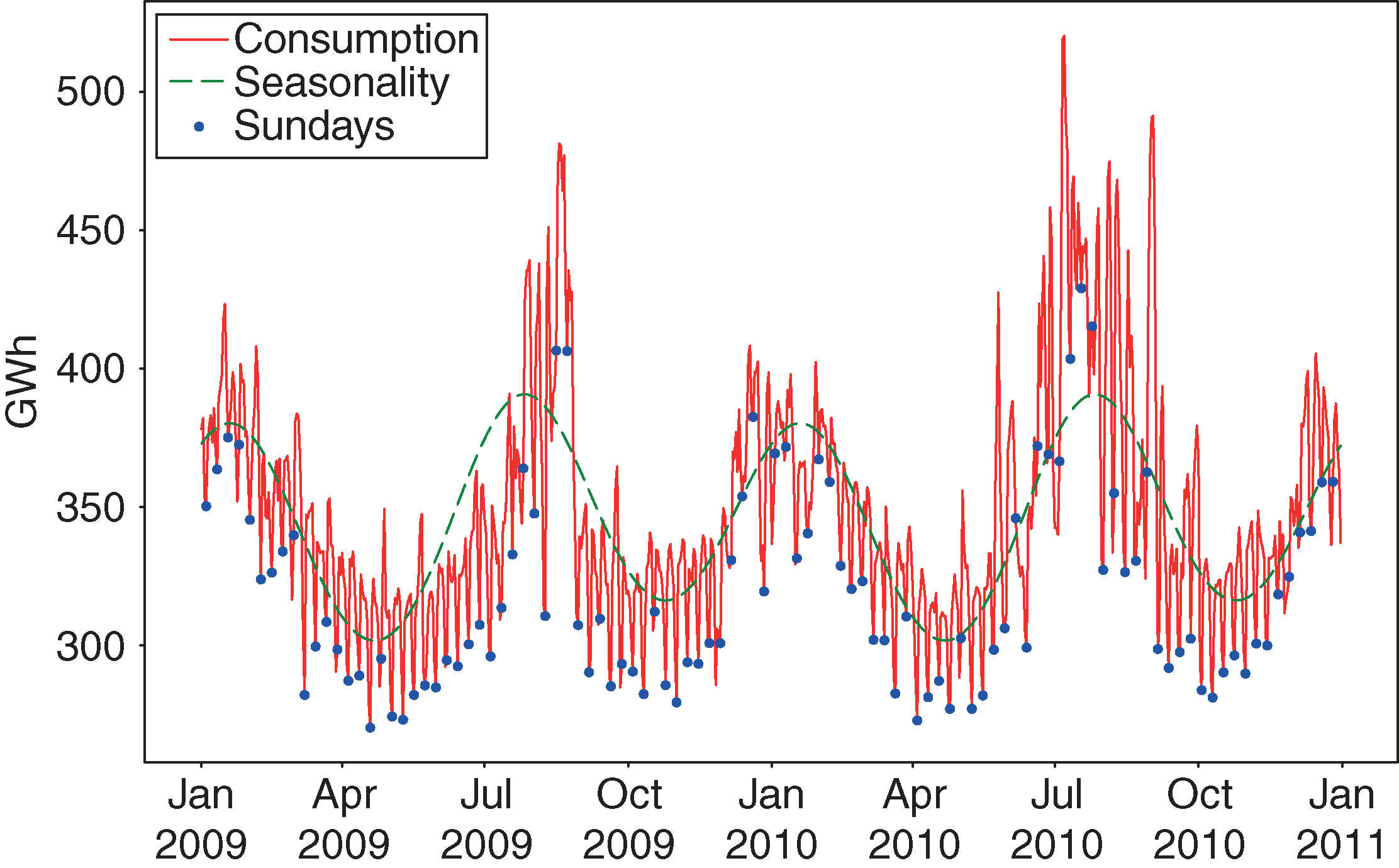
We observe that

1. (i)

   power consumption in summer is double the power consumption during spring or fall,

2. (ii)

   consumption on weekdays is higher than on Sundays, and

3. (iii)

   volatility and spikes are larger during summer than the rest of the year.

These are well-known stylized facts common to most households’ electricity consumption time series, specifically in regions where there is massive use of air-conditioning during summer and a significant source of heat comes from heat pumps during winter. For these reasons, and due in particular to the seasonality in the observed volatility, it is now standard in the literature to model the logarithm of households’ electricity consumption (for a review, see, for example, Hong and Fan (2016)).

In the next section, we describe the adopted methodology in detail.

3 Methodology

3.1 The model

Most of the forecasting studies on the power market focus on price forecasting (for a review, see, for example, Nowotarski and Weron 2018); in this paper, we focus on a middle-term density forecast for power consumption, where the number of studies in the literature is rather limited (see, for example, Hong and Fan 2016).

We aim to forecast future power consumption over the middle-term horizon, modeling both seasonal and weather-related features; the goal is to obtain a density forecast of daily consumption with a reasonably simple description.

As already mentioned in the previous section, we model log-scaled daily electricity consumption data, as this is standard in the literature for probabilistic forecasting in the energy sector. The characteristics of the power demand we desire to model are the long-term trend and seasonal behavior (both yearly and weekly) as well as the daily autocorrelation, the relation with weather conditions and variance clustering.

We build a hybrid model composed of two blocks: a linear model that describes trend and seasonality, and an NN that describes the weather influence and the nonlinear effects of seasonality (eg, the calendar effect on the variance).

A hybrid model approach, where we separate first trend and seasonality and then analyze the residuals separately, is standard in the energy literature (see, for example, Benth et al (2008) and the references therein). First, the relation between the logarithm of consumption and calendar variables is established through a general linear model (GLM). Then, we investigate the relationship between GLM residuals and weather variables through a shallow NN.

The GLM part of the model is elementary. We model the natural logarithm of power consumption $Y_t$ as

$$Y_t=T_t+S_t+R_t,$$

(3.1)

where

	$T_t$	$={\beta }_0+{\beta }_{1}t,$
	$S_t$	$={\displaystyle \sum _{k=1}^2}[{\beta }_{1+k}\sin (k\omega t)+{\beta }_{2+k}\cos (k\omega t)]$
		$\mathrm{\hspace{1em}\hspace{1em}}\mathit{\hspace{1em}\hspace{1em}\hspace{1em}\hspace{1em}\hspace{1em}\hspace{1em}}+{\beta }_6{D}_{\mathrm{Sat}}(t)+{\beta }_7{D}_{\mathrm{Sun}}(t)+{\beta }_8{D}_{\mathrm{Hol}}(t),$

and calendar time is measured via the cardinality $t$ of the observation, starting from 0 on the first date in the data set; $R_t$ are the residuals, $T_t$ is the trend term and $S_t$ is the seasonality (both yearly and weekly). For the yearly seasonality, we use both annual and semiannual seasonality terms with $\omega :=2\pi /365$; these sinusoidal terms with order $k\le 2$ describe the two peaks per year observed in Figure 2. Moreover, the holidays’ contribution is modeled with a dummy variable. The weekly seasonality is introduced via two dummy variables for Saturday and Sunday.

Figure 3: The (a) autocorrelation and (b) partial autocorrelation functions of seasonally adjusted consumption time series in the time window 2007–10. We observe that the time series is autocorrelated; from the partial autocorrelation, we note that the time series is at least AR(1).

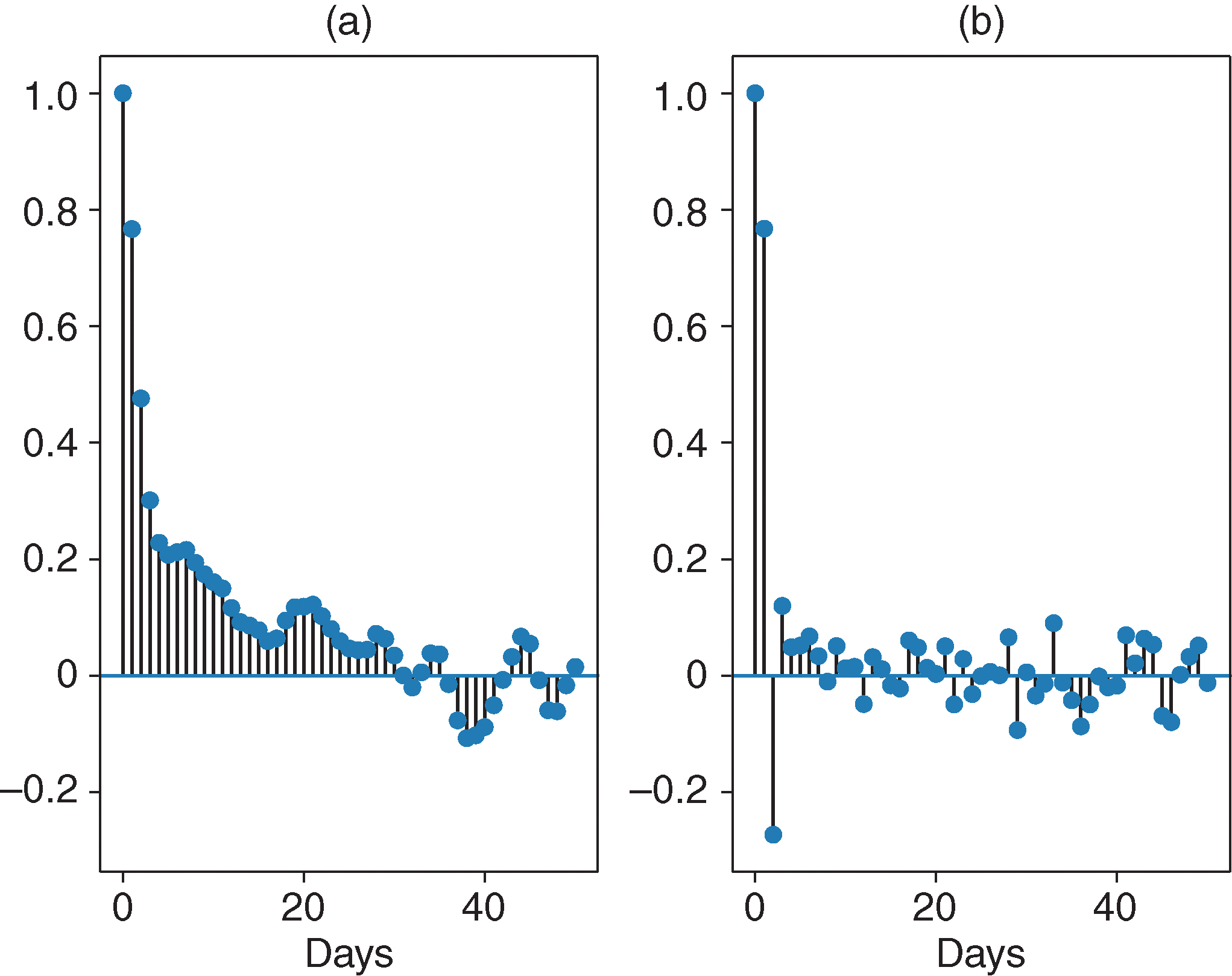
We measure the autocorrelation and the partial autocorrelation of the residuals $R_t$ on the time window 2007–10; Figure 3 highlights the necessity of a one-day autoregressive component. Further, the augmented Dickey–Fuller test rejects the null hypothesis of a unit root for the deseasonalized time series.

The residuals $R_t$ are modeled via an NN. NNs are generally used for point forecasting, where they can achieve excellent results. However, the literature on probabilistic forecasting of electrical consumption with NNs is scarce. As already mentioned in Section 1, as yet there is only one study available: Vossen et al (2018) use a standard feed-forward NN (FFNN) for density forecasting.

An FFNN represents the most standard and straightforward type of NN. Its name arises from the fact that, in this structure, the information moves only in one direction (forward) from the input layer, through the hidden neurons and finally to the output layer. Further, if we were to represent an FFNN architecture with a computational graph, where each node represents a neuron and each edge represents the information flow between two neurons, we would see that those connections do not form any cycle.

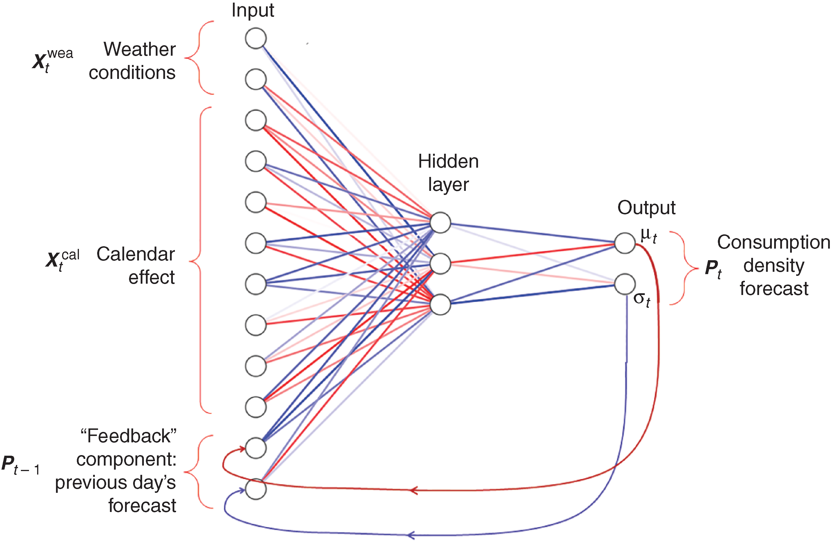
However, because the time series analyzed show a significant one-time-step autocorrelation, we consider an NN with an “autoregressive” feature: the NN outputs at time $t-1$ are used as two additional inputs to the NN for the next time in the series. This feature resembles the structure of a recurrent NN, where the output of a given layer is considered as an input to the same NN layer (see, for example, Rodrigues et al 2014; Kong et al 2017); in this paper, we consider only feedback from the output layer into the input layer. This rather simple architecture is shown in Figure 4. This construction replicates the “autoregressive” feature in standard autoregressive (AR) models. Because the structure resembles that of autoregressive exogenous (ARX) models, we call the proposed hybrid model an NN with autoregression and exogenous inputs (NAX). In the next subsection, we describe in detail the NN part of the model.

Figure 4: Schematic of the NAX model selected in the validation procedure. Note the twelve-dimensional input (two weather conditions ${?}_t^{\text{wea}}$, eight neurons for the calendar effects ${?}_t^{\text{cal}}$ and two autoregressive terms ${?}_{t-1}$), a three-neuron hidden layer and a two-dimensional output ${?}_t$ with two components (${\mu }_t$ and ${\sigma }_t$).

3.2 Neural network with autoregression and external inputs

It is well known that, after having detrended and deseasonalized the time series, the impact on power consumption of weather conditions in general, and of temperature in particular, cannot be neglected (see, for example, Hong and Fan 2016).

In this paper, the residuals of power consumption are modeled via a simple NN with a feedback from the output to the input. Moreover, following the promising results obtained by Gaussian processes in probabilistic forecasting of power consumption (see, for example, Baviera and Messuti 2020), we consider the residuals $R_t$ to be normally distributed with unknown mean ${\mu }_t$ and variance ${\sigma }_t^2$. The main contribution of this study from a modeling perspective is the consideration of an NN with the following three characteristics:

1. (i)

   it presents a two-dimensional output vector that models time-dependent density parameters,

2. (ii)

   it presents an “autoregressive” structure with NN output included as the input at the next time step, and

3. (iii)

   it incorporates information from weather conditions and calendar effects.

Figure 4 describes an example of the NAX structure; we observe a vector output ${?}_t$ with two components (${\mu }_t$ and ${\sigma }_t$) and inputs at time $t$ that include both the exogenous inputs (${?}_t$) at time $t$ and the outputs (${?}_{t-1}$) at time $t-1$.

The NN we consider has $I$ exogenous inputs (including both weather conditions and calendar effects) and one hidden layer with $N$ neurons.⁴⁴ 4 Note that, in this case, the NN reduces to a recurrent NN with one nonlinear hidden layer and one linear output layer. Thanks to the simplicity of the structure, it is possible to describe this NN with the following equation:

$${?}_t=L\mathscr{H}(?{?}_t+?{?}_{t-1}+{?}_0)+L_0,$$

(3.2)

where $\mathscr{H}$ is the nonlinear activation function (eg, softmax, sigmoid), a vector in ${ℝ}^N$; $L$ is a $2\times N$ array of weights for the output of the $N$ neurons in the hidden layer, while $L_0$ is the two-dimensional bias on the output; $?$ is the $N\times I$ array of weights for the input of the $N$ neurons in the hidden layer, while ${?}_0$ is the $N$-dimensional vector of bias on the $N$ neurons; and $?$ is the $N\times 2$ array of weights of the feedback term of the $N$ neurons.

Our analysis is divided into four main steps, the first three in line with the NN literature (see, for example, Ripley (2007) and the references therein), and a fourth to evaluate the robustness of the proposed solution. We implement the NAX in Keras with TensorFlow backend (see https://keras.io). To avoid the problem of different input and output scales, we normalize all the input and output data with the min–max normalization technique (see, for example, Patro and Sahu 2015, p. 1) before feeding them into the NAX. Every column of the data matrix is standardized and destandardized using only information in the training set.

First, we train the NAX maximizing the Gaussian likelihood function as proposed by Vossen et al (2018, eq. 2), where

$$L({\mu }_t,{\sigma }_t\mid R_t)=\frac{1}{\sqrt{2\pi {\sigma }_t^2}}\exp \left(-\frac{{(R_t-{\mu }_t)}^2}{2{\sigma }_t^2}\right)$$

is the likelihood function for the residual $R_t$ in (3.1).⁵⁵ 5 Note that the NAX outputs are a direct estimation not of the residual $R_t$ but of the two parameters ${\mu }_t$ and ${\sigma }_t$. When training the NN we look for the parameters that maximize the likelihood of the realized residuals in the training set.

Figure 5: An example of the time line describing the data segmentation we use to validate (above the time axis) and test (below the time axis) the NAX model. The length of the training window (in years) is a hyperparameter; we train on the years before 2011 and select the best model hyperparameters on the validation set (2011). In particular, we show the case of a three-year training set (2008–10). Then, for testing, we calibrate the selected model on the years before 2012 (keeping the training set length equal to the selected hyperparameter), and we test the performance of the model on 2012 data.

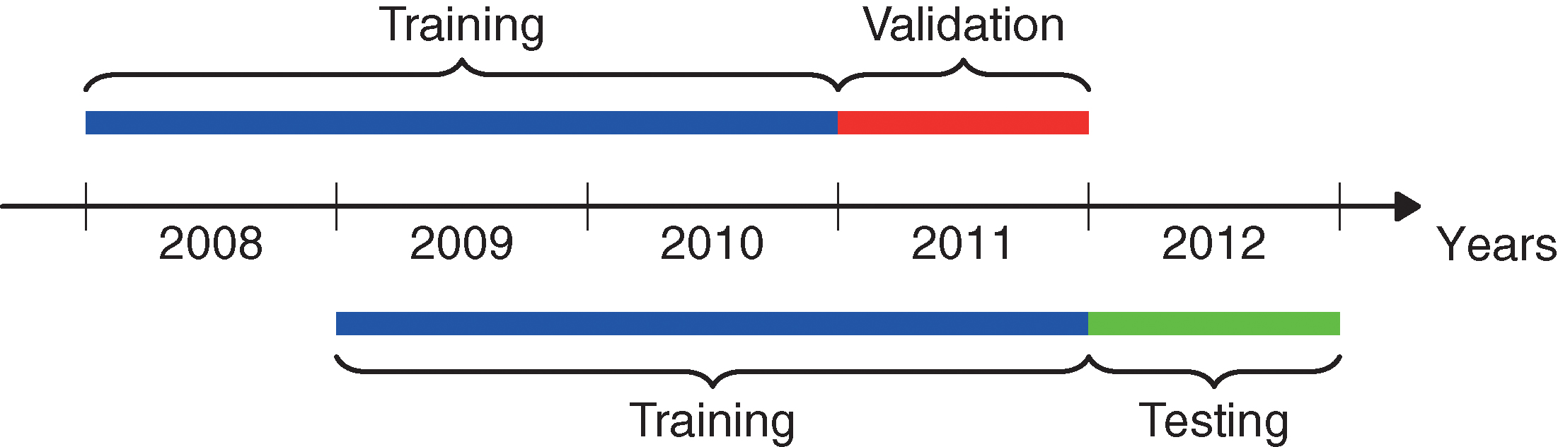
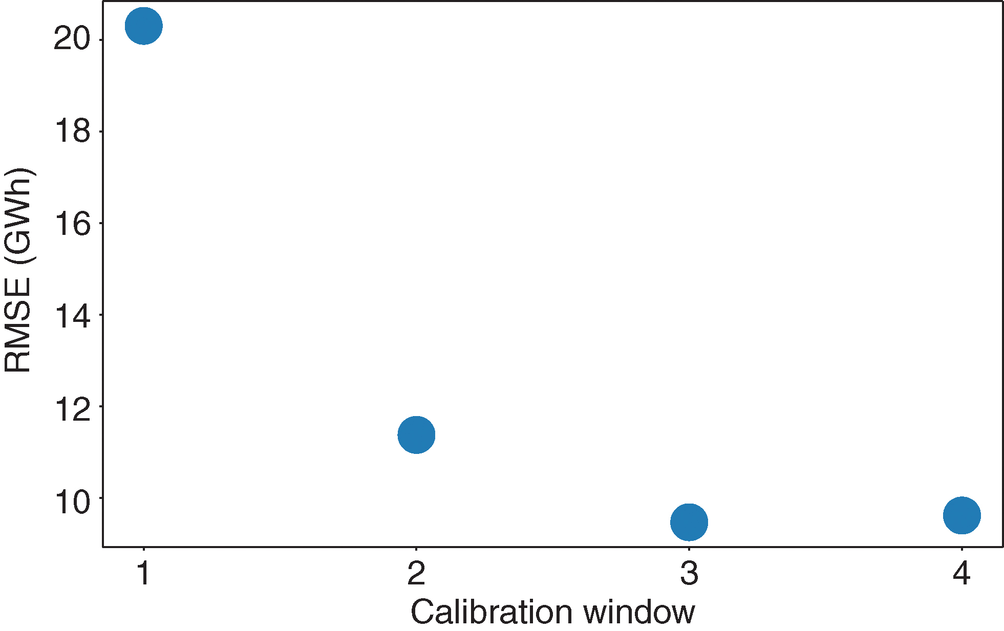
Second, we select the hyperparameters of the NAX model. We perform a grid search on the hyperparameters on the validation set (the year 2011). Figure 5 describes the data segmentation in the training, validation and testing sets. The NAX model is trained on the training set for every possible combination of the hyperparameters in Table 2, and the model with the smallest root mean squared error (RMSE) on the validation set is selected. Minimizing RMSE is standard among power suppliers: this helps to focus calibration on periods of higher consumption, often characterized by higher electricity costs. Even if we estimate the network with respect to the Gaussian likelihood (in order to estimate the consumption density), we decided to select the model that satisfies this industry requirement. In this study, the training set time window length is one of the hyperparameters. As already discussed in Section 1, due to the rapid changes that are observed in the power market, it is important to avoid training on years that do not help the NN in its ability to generalize: it has been selected as the longest time window for which we observe a decreasing RMSE in the validation set.

Figure 5 shows an example of the data segmentation we use to validate the NAX model (compared with the training and validation sets above the time axis): in particular, in the figure we consider the case when the training set time window is three years.

Table 2: Set of hyperparameters analyzed in the validation step.

Hyperparameter	Values
Number of neurons (hidden layer)	3, 4, 5, 6, 8, 10
Activation function	softmax and sigmoid
Initial learning rate	0.1, 0.01, 0.001, 0.0007, 0.0005, 0.0001
Batch size	50, 100, 350, no batch
Regularization parameter	0.01, 0.001, 0.0001, 0
Training set time window	1, 2, 3 and 4 years

Third, we consider the test set (the year 2012), on which we perform the model evaluation according to a set of indicators. Figure 5 shows an example of the data segmentation we use to test the NAX model (compare the training and testing sets below the time axis): we train the selected model on the three years before 2012 (the training set length is equal to the selected hyperparameter) and test the performance of the model on 2012. Both validation and testing are conducted via an ex post probabilistic forecasting of power consumption, standard in middle-term forecasting. The next subsection describes in detail the ex post density forecasting technique and the evaluation methods we consider in probabilistic forecasting.

Finally, in addition to the three classical steps, we perform a robustness test to verify the quality of the proposed hybrid model: we evaluate model performances in the years 2013–16 (see also Figure 1), training the model with the same hyperparameters as selected in the validation set. The results are summarized in Section 4.

3.3 The ex post forecasting technique and the evaluation methods

The probabilistic forecasting of middle-term daily power consumption is obtained via ex post forecasting. This technique, introduced by Hyndman and Fan (2010) in the power consumption sector, is commonly used in middle- to long-term power consumption forecasts (see, for example, Goude et al 2013). The model we consider is divided into three stages (see, for example, Hyndman and Fan 2010, p. 1144), shown in the flow diagram in Figure 6: calibration, forecasting and evaluation. The first stage is applied to the in-sample (training) set. The second and third stages use the out-of-sample set: this can be either the validation set or the test set, depending on whether we are selecting the optimal hyperparameters or we are testing the model.

Figure 6: Flow-diagram of the three stages of the ex post technique: calibration, forecasting and evaluation of the proposed model. The presence of a forecasting stage is the main difference with respect to the standard technique.

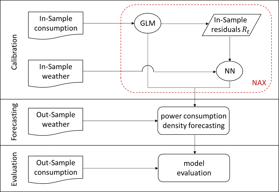
In the calibration stage, the NAX model, with its two components (GLM and NN), is trained on the in-sample set with both power and meteorological data. The GLM is calibrated through ordinary least squares and the NN is trained using the Keras ADAM optimizer.

In the forecasting stage, the density is estimated via an ex post forecast. This second stage is the main difference from standard forecasting. Our forecast uses the weather conditions in the out-of-sample set to forecast the power consumption; as explained by Goude et al (2013, p. 443), it “allows us to quantify the performances of our model without embedding the meteorological forecasting errors”. The idea is that, to focus on the ability of the model to describe a strong and reliable relationship between temperature and power consumption, we suppose that the temperatures in the out-of-sample period are known. With the proposed model, ex post forecasting is straightforward.

Finally, in the evaluation stage, the quality of the model forecast is evaluated by comparing it with the out-of-sample realized test consumption data. The model is evaluated both in terms of point consumption forecasting and in terms of the sharpness and reliability of the predicted densities.

In addition to the standard measures of point consumption forecasts, such as RMSE and mean absolute percentage error (MAPE), we provide some evaluation methods for density forecasting. When dealing with density forecasting, it is more difficult to value the quality of the forecast. We are not able to observe the realized distribution of the underlying process: we cannot compare the predicted distribution with the true one, as we only have one realization for each distribution. The evaluation is based on two main measures: the sharpness, which verifies the tightness of the density forecasting, and the reliability, which tests the distribution’s statistical significance (for a detailed description, see Nowotarski and Weron (2018) and Baviera and Messuti (2020) and the references therein). Let us briefly summarize their main characteristics.

Sharpness is measured via the pinball loss function. This is an error measure for quantile forecasts. The pinball allows both a qualitative and a quantitative comparison of models. In the former, a symmetric pinball loss denotes that the density forecast reflects the right and left tails of the true distribution with the same precision, while in the latter, to quantitatively assess the sharpness, we compute the average of the pinball loss (APL) over 99 percentiles (from 1% to 99%); APL was the quantitative measure used to rank models in the 2017 GEFCom competition (see, for example, Hong et al 2016).

Reliability measures the consistency of the predicted distribution with the realized observations and the robustness of the performance of the selected configuration of hyperparameters over time. The former is verified via backtesting of the confidence intervals (CIs), eg, if 90% of the realized observations fall within the predicted 90% CI, then this CI is considered reliable. From a quantitative point of view, unconditional coverage tests this zero hypothesis. Moreover, conditional coverage tests the zero hypothesis that failures of the CI are not clustered together in the time series. The latter is checked, as described in the fourth step of Section 3.2, via the measure of some performance indicators both for point forecasting and for density forecasting over four years (2013–16), keeping the optimal hyperparameter configuration chosen in the validation step. In the next section, we summarize the main results.

4 Results

In the previous section, we discussed the three stages of the analysis for both model validation and testing, after data preprocessing: calibration, forecasting and evaluation (see Figure 6). Preprocessing the data consists in the treatment of leap years and outliers. We remove February 29 data from the data set in leap years, while outliers are treated as in Benth et al (2008): in the 2007–10 training set, no outlier is detected.

For validation, we train the NAX on every combination of the hyperparameters reported in Table 2. In particular, we select the training set time window: as already mentioned, this is a relevant hyperparameter because the power market is rapidly evolving. It is crucial to train the NN on a time interval that helps its ability to generalize. Starting from one year, we consider longer intervals in yearly steps: we notice an improvement on extending the training window to three years, while the RMSE is higher for the four-year time window. Figure 7 compares the RMSEs on the validation set (2011) of the best selected model by varying the length of the training window.

The best-performing configuration on the validation set is the one with three neurons in the hidden layer, softmax activation, a three-year training window, an initial learning rate of 0.003, a batch size of 50 observations and a regularization parameter equal to ${10}^{-4}$. Moreover, we compare the NAX model with two simple benchmarks in the power industry: the GLM (the simplest benchmark model, which does not include any weather information) and the ARX model (see, for example, Box et al 2015, pp. 534ff), where an autoregressive component appears among the linear regression covariates together with weather conditions and calendar effects (as exogenous variables). For comparison, we also consider another machine learning approach: a Gaussian process with exogenous inputs (GPX) (see, for example, Baviera and Messuti 2020). Of all the models analyzed, the selected NAX is the best performer in the validation set.

Figure 7: The RMSE of the validation set (2011) with a training window of one year (2010), two years (2009, 2010), three years (2008–10) and four years (2007–10). For every time window, we show the RMSE of the best of the calibrated models. We notice an improvement by extending the training window up to three years.

For testing, the NAX model is calibrated on the new training set (from January 1, 2009 to December 31, 2011), first by fitting the GLM and then by training the NN. The GLM parameters calibrated on the 2009–11 time window are reported in Table 3.

Table 3: GLM parameters calibrated on the training data set 2009–11 with their standard deviation (SD). [${}^{***}$Statistical significance of the parameters at a 1% significance level.]

		Estimate	SD
Intercept	${\beta }_{\text{0}}$	$-$0.385${}^{***}$	(0.023)
Trend	${\beta }_{\text{1}}$	$-$0.16${}^{***}$	(0.04)
$\text{sin}(\omega t)$	${\beta }_{\text{2}}$	$-$0.003	(0.004)
$\text{cos}(\omega t)$	${\beta }_{\text{3}}$	$-$0.028${}^{***}$	(0.004)
$\text{sin}(\text{2}\omega t)$	${\beta }_{\text{4}}$	$-$0.136${}^{***}$	(0.004)
$\text{cos}(\text{2}\omega t)$	${\beta }_{\text{5}}$	$-$0.043${}^{***}$	(0.004)
Saturday	${\beta }_{\text{6}}$	$-$0.120${}^{***}$	(0.008)
Sunday	${\beta }_{\text{7}}$	$-$0.146${}^{***}$	(0.008)
Holiday	${\beta }_{\text{8}}$	$-$0.060${}^{***}$	(0.016)

Figure 8: ARX and GPX power consumption middle-term prediction.. Realized (dashed green line) and expected (red line) power consumption in GWh between January and December 2012 with predicted 95% CI (shaded area). (a) ARX. (b) GPX.

Figure 9: NAX power consumption middle-term density prediction. Realized (dashed green line) and expected (red line) power consumption in GWh between January and December 2012 with predicted 95% CI (shaded area). We observe that, in terms of point forecasting, the model is able to provide a precise forecast even if there are spikes in consumption over summertime; in terms of density, realized consumption falls within the 95% CI on all but 15 days (95.8% of cases).

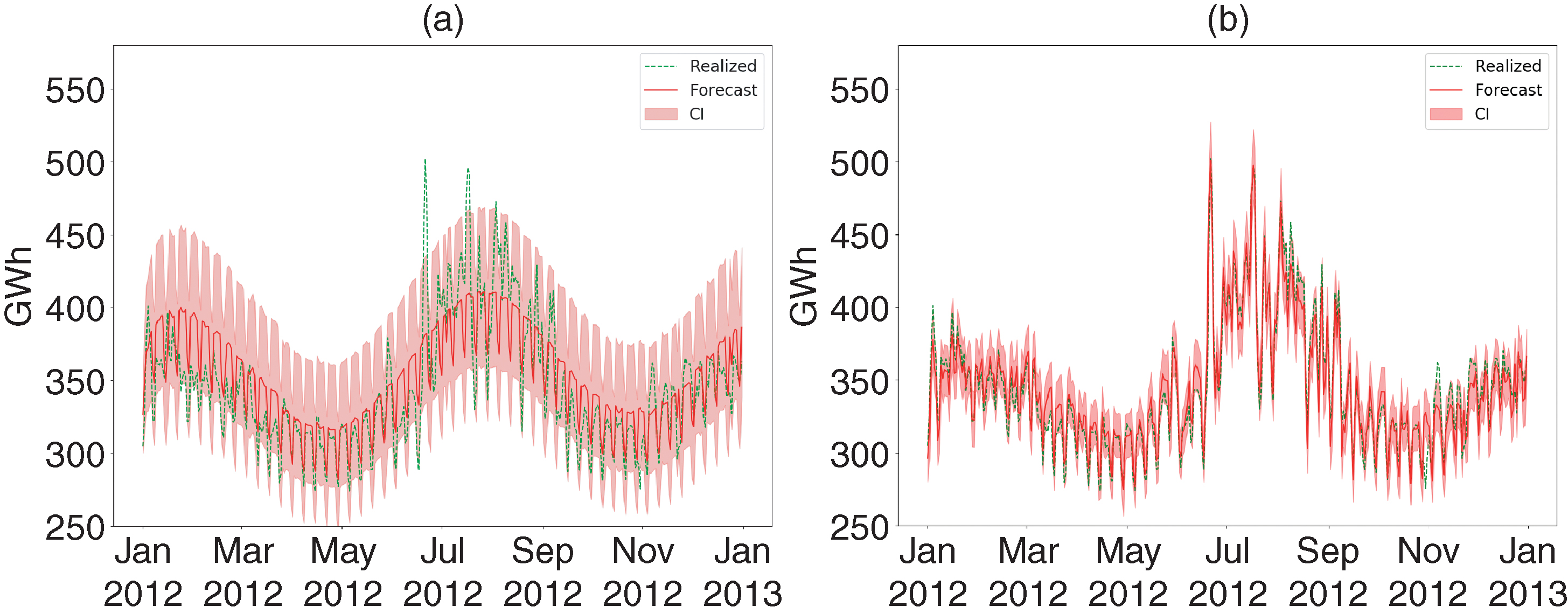
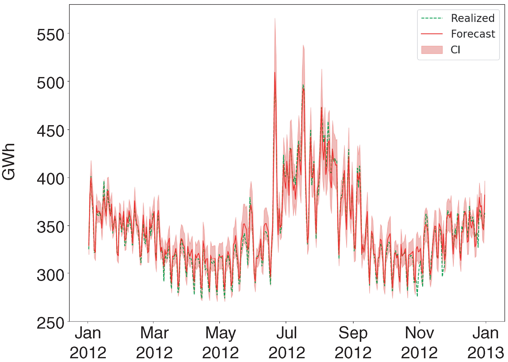
Ex post forecasting with the four models is straightforward. We evaluate each model both qualitatively and quantitatively. From a qualitative perspective, we plot the models’ forecast on the test set: we consider ARX and GPX in Figure 8, while in Figure 9 we show the performance of NAX. The solid (red) line indicates the point forecast, while the lighter shaded area indicates the 95% CI; the dashed (green) line shows the power consumption realized on the test set. We observe that GPX improves the ARX performance significantly in terms of both point and density forecasting, but it is less accurate than NAX. In particular, ARX CIs look quite large. As regards the NAX model, even if each density forecast at time $t$ is a simple Gaussian with mean $T_t+S_t+{\mu }_t$ and variance ${\sigma }_t^2$, the results in Figure 9 look impressive: not only does the point forecast track closely the realized consumption (even the spikes in the summertime are tracked accurately), but also the realized consumption falls within the 95% CI on all but 15 days (95.8%), and the densities reproduce the observed behavior of periods of high volatility in summertime followed by periods of low volatility in wintertime.⁶⁶ 6 Let us highlight that the last power consumption date considered in the model calibration is December 31, 2011, while the forecasting goes up to one year later, ie, to December 31, 2012.

In the remainder of this section, we discuss some quantitative criteria that show the quality of both the point and the density forecasts, comparing the results with those of GLM, ARX and GPX. We first consider accuracy measures for the point forecast, and then we show the results for the sharpness and reliability of the probabilistic forecast: these evaluation techniques were described in Section 3.

Table 4: RMSE and MAPE for the four models considered on the test set (2012). [We observe that the NAX error metrics (in boldface) are the most accurate. The NAX presents an MAPE of less than 5% (ie, it is considered a good forecast by practitioners), and the lower absolute error (RMSE) indicates a more precise point forecasting in summertime (ie, when forecasting is more relevant due to the spikes in consumption).]

	GLM	ARX	GPX	NAX
RMSE (GWh)	26.69	26.13	10.74	8.10
MAPE (%)	06.00	05.80	02.50	1.74

First, we compute the RMSE and MAPE of the point forecasting on the test set (see Table 4). We can note that GPX and NAX are significantly better than GLM and ARX in terms of the RMSE and MAPE, with NAX being the best. In particular, both GPX and NAX are below the 5% threshold that characterizes good power forecasting models for practitioners. Moreover, a lower RMSE (more than two-thirds lower than GLM and almost one-third lower than GPX) indicates that NAX also reduces the error significantly in summertime, when the forecasting is more relevant due to higher consumption and volatility: a behavior we observe in Figures 8 and 9.

Second, we analyze the sharpness. Figure 10 represents the pinball loss for the four models on every percentile. We observe that for all percentiles (with one exception) the NAX pinball loss is significantly lower than the other three models’ pinball loss.

Figure 10: Pinball loss functions for the four models for every percentile. We observe not only that NAX presents the lowest score for all percentiles (ie, it is sharper and more accurate), but also that the pinball loss is symmetric for both NAX and GPX.

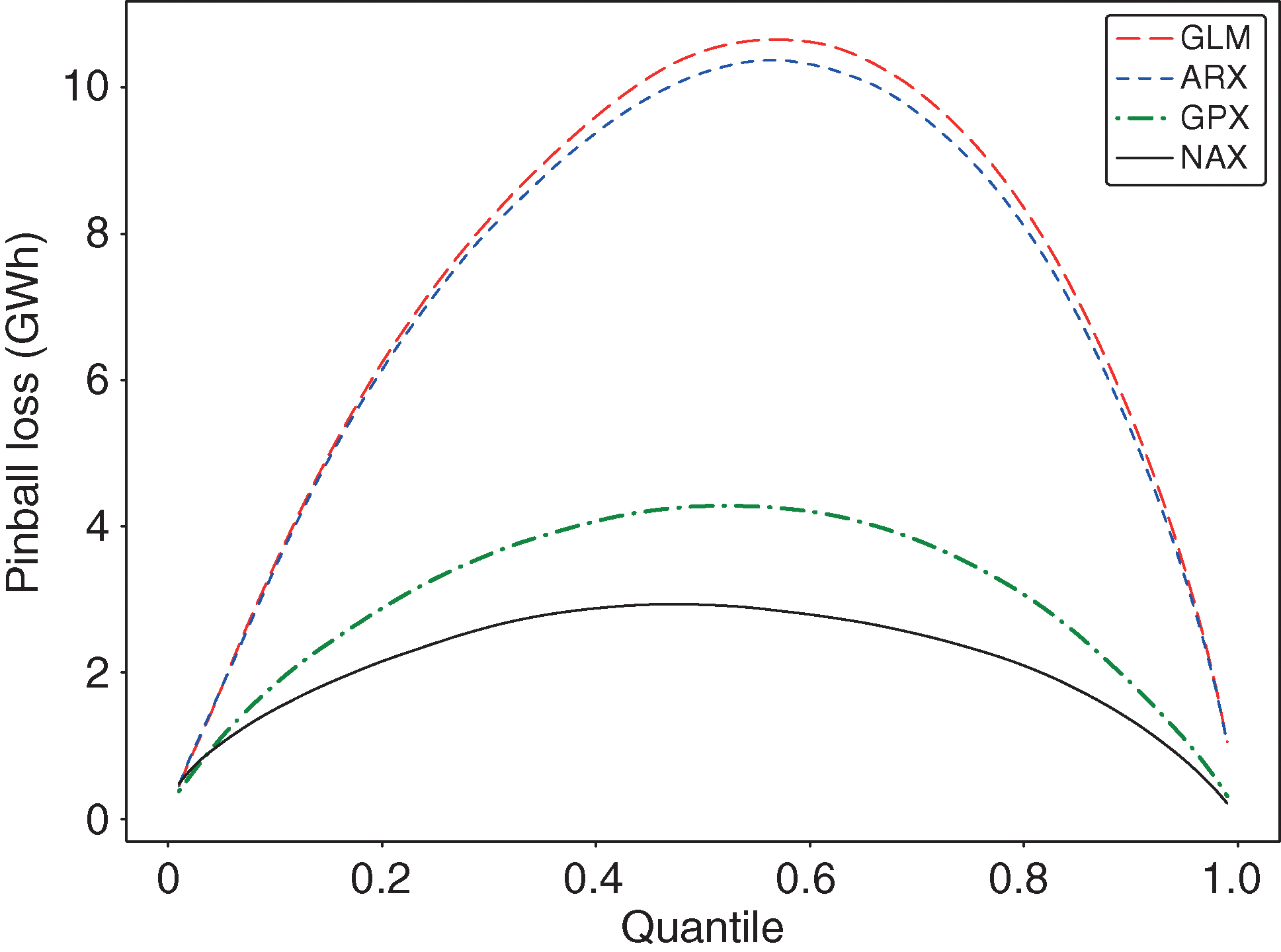
The plot of the pinball loss provides useful information not only in terms of sharpness but also related to its symmetric shape: density forecasting of power consumption, for both NAX and GPX, reproduces with a similar accuracy both the right and the left tails of the actual consumption density. NAX appears to be the most accurate, having the lowest pinball loss.

Finally, we test model robustness by both backtesting the CI and verifying its reliability over time. First, we backtest CI, counting the fraction of days the realized power consumption falls outside a confidence level $\alpha$ of the predicted density (violations) and comparing this with the nominal ones, equal to $1-\alpha$. We can observe in Figure 11 that the NAX backtested CIs are close to the nominal values. GLM and ARX backtested quantiles look better but this is due to the fact that the CIs are much larger: one must take into account the sharpness of NAX and GPX CIs compared with the linear benchmarks (see Figures 8 and 9). In any case, both GPX and NAX provide good results.

Figure 11: Backtested CIs. We show the fraction of times the realized power consumption falls inside a confidence level $\alpha$ against $\alpha$. We observe that the empirical coverage for GPX and NAX is very close to the nominal levels for high quantiles, with NAX being significantly better than GPX.

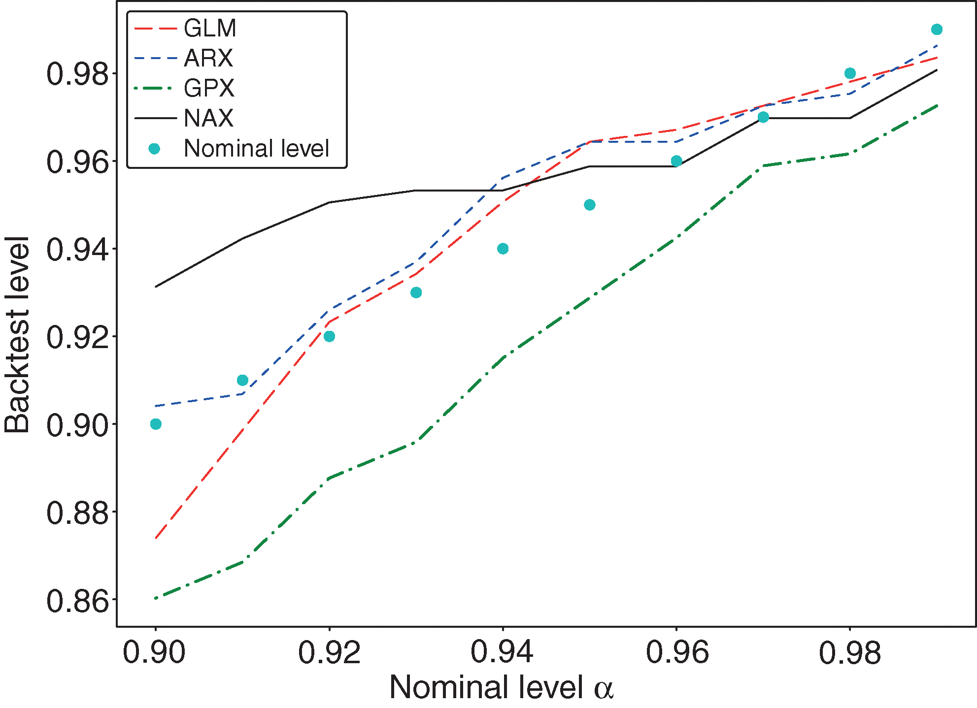
These results on the CIs are also tested from a quantitative point of view through likelihood ratio tests. Table 5 outlines the results of these unconditional coverage and conditional coverage tests, which became standard in the backtesting of value-at-risk in the banking industry after the introduction of Basel II. The unconditional coverage is a test on the number of violations, while the conditional coverage tests whether violations tend to cluster in some particular periods. All models pass the unconditional coverage test, but none passes the conditional coverage. This result suggests we analyze the time series of violations in more detail; we can observe that, for the NAX model, violations cluster only in the fall and spring (which causes the test failure), while in winter and summer, ie, the most interesting periods for power forecasting, the violations are distributed regularly.⁷⁷ 7 This analysis is available from the authors upon request.

Table 5: Likelihood ratio tests at a 95% level of the 95% CI. [The ${\chi }^{\text{2}}$ test statistic represents the threshold over which the null hypothesis should be rejected.]

	GLM	ARX	GPX	NAX	${?}^{\text{?}}$
Unconditional coverage	01.76	01.76	03.08	00.63	3.84
Conditional coverage	27.28	27.28	13.86	22.84	5.99

Then, to verify the robustness of the NAX and the GPX performance over time, we evaluate the forecasts on the years from 2013 to 2016; we consider a NAX model with the same hyperparameters as selected in the validation step, and we calibrate the model parameters only on the new training set time window (eg, 2010–12 for the year 2013). This analysis is particularly relevant for machine learning techniques that involve several hyperparameters. Table 6 compares the MAPE, RMSE and APL of GPX and NAX on the different test sets (from 2012 to 2016). In every year, the MAPE falls well below the 5% threshold; NAX always performs better than GPX (except for the 2015 testing year) in terms of both point and density forecasting.⁸⁸ 8 Note the differences between the two modeling approaches. While for GPX there is a standard model calibration of model parameters on the three-year calibration period, for NAX we consider the same hyperparameters as those selected in the validation and we are just training model weights.

Table 6: The MAPE, RMSE and APL for GPX and NAX on different test sets (from 2012 to 2016). [We observe that the NAX and GPX in all testing years give an MAPE of less than 5%. The MAPE values are stable, and NAX always has the best MAPE, RMSE and APL (except for in the 2015 testing year).]

	MAPE (%)		RMSE (GWh)		APL (GWh)
	GPX	NAX	GPX	NAX	GPX	NAX
2012	2.50	1.74	10.74	08.10	3.04	2.15
2013	2.17	2.13	10.30	10.10	2.82	2.76
2014	2.39	2.00	10.66	08.70	2.95	2.49
2015	2.41	2.52	10.31	10.74	2.93	3.05
2016	3.16	1.70	13.46	07.58	3.94	2.07

In summary, Table 6 and Figure 11 show the strongest results of our analysis. On the one hand, Figure 11 shows that the proposed model accurately reproduces the observed tail distribution with a frequency of violations close to the nominal level: not only do we have an MAPE of less than 5% over the whole time horizon, but the nominal level and the empirical coverage appear to be close for all values of $\alpha$. On the other hand, Table 6 shows that the NAX model can provide robust point and density forecasts for daily power consumption over time, even without changing the optimal model hyperparameters.

5 Ex ante prediction

In the previous section, we evaluated the model density forecasting performance using realized temperature data (ex post forecasting); as already discussed, this is the most relevant piece of information for both academics and practitioners, because it is linked to the ability of the model to describe reliably the strong relationship between temperature and power consumption, even on a middle-term horizon, without embedding forecasting errors in temperatures.

One possible application is to verify also the ex ante prediction power of NAX in a real-world situation by simulating the daily temperatures on the tests set (2012).⁹⁹ 9 We thank a referee for suggesting this application. An analytical formula for the cumulative distribution function (CDF) for the ex ante residual $R_t$ can be obtained by conditioning on the temperature time series. For every $K\in ℝ$, we have

where $?$ is the random time series of the daily temperatures, $?[\cdot ]$ is the expectation with respect to the simulated temperature $?$, and $N(\cdot )$ is the CDF of a standard normal random variable. NAX provides the conditional CDF given the time series $?$: ${\mu }_t(?)$ and ${\sigma }_t(?)$ are the NAX outputs computed by considering the temperatures $?$ as inputs. We can estimate the cumulative distribution by giving the same probability to every simulated temperature time series.

For the temperature simulation, we follow the approach introduced by Hyndman and Fan (2010, pp. 7–8). One bootstrapped temperature sequence consists of a sample of blocks of length $L$ randomly selected with a uniform distribution in $(m-\mathrm{\Delta },m+\mathrm{\Delta })$. The block comes from a different (previous) randomly selected year (between 2007 and 2011), and a random shift $S$ uniform in $(-\mathrm{\Delta },\mathrm{\Delta })$ is applied to the days of the year. We select $m=7$ and $\mathrm{\Delta }=3$, and we simulate 2000 paths as in Hyndman and Fan (2010, p. 9). For example, we start the bootstrapped time series from January 1, with a block 1 of seven days, and this block may come from 2010; block 2 can have $L=9$ and $S=1$, and the nine-day block may come from the period starting on January 9, 2009, and so on, up to December 31. Unlike Hyndman and Fan (2010), we do not add any additional noise to the temperatures to closely match those observed in the time window we consider.

We can then evaluate the quality of the obtained ex ante forecast. First, we compare the RMSE and MAPE of ex post and ex ante point forecasting in Table 7. As expected, we observe an increase in the point forecasting error.

Table 7: The RMSE and MAPE for ex ante and ex post forecasts on the test set (2012). [As expected, we observe larger errors for the ex ante forecast because we consider the uncertainty in temperatures.]

	Ex ante	Ex post
RMSE (GWh)	28.99	8.10
MAPE (%)	06.01	1.74

Figure 12: NAX power consumption ex ante middle-term density prediction. Realized (dashed green line) and expected (solid red line) power consumption in GWh between January and December 2012 with predicted 95% CI (shaded area). We observe that the model can provide a valid ex ante point forecast, but it misses some spikes in summer and winter; in terms of density, the realized consumption falls within the 95% CI on all but 22 days (94.0% of cases). The CI appears to be wider than in the ex post case (cf, Figure 9).

Figure 13: Ex post (solid black line) and ex ante (dashed red line) forecasted densities for (a) January 15, (b) April 15, (c) July 15 and (d) October 15, 2012. In all cases, we observe a wider distribution in the ex ante forecast, and the realized consumption falls within the densities. The seasonality of volatility is preserved. Note that the ex ante distributions are significantly wider in summer and winter, while during spring and fall the two densities appear quite close.

Figure 14: Backtested CIs. We show the fraction of times the realized power consumption falls inside a predicted confidence level $\alpha$ against $\alpha$. We observe that the empirical coverage for ex ante and ex post predictions is close to the nominal levels for high quantiles.

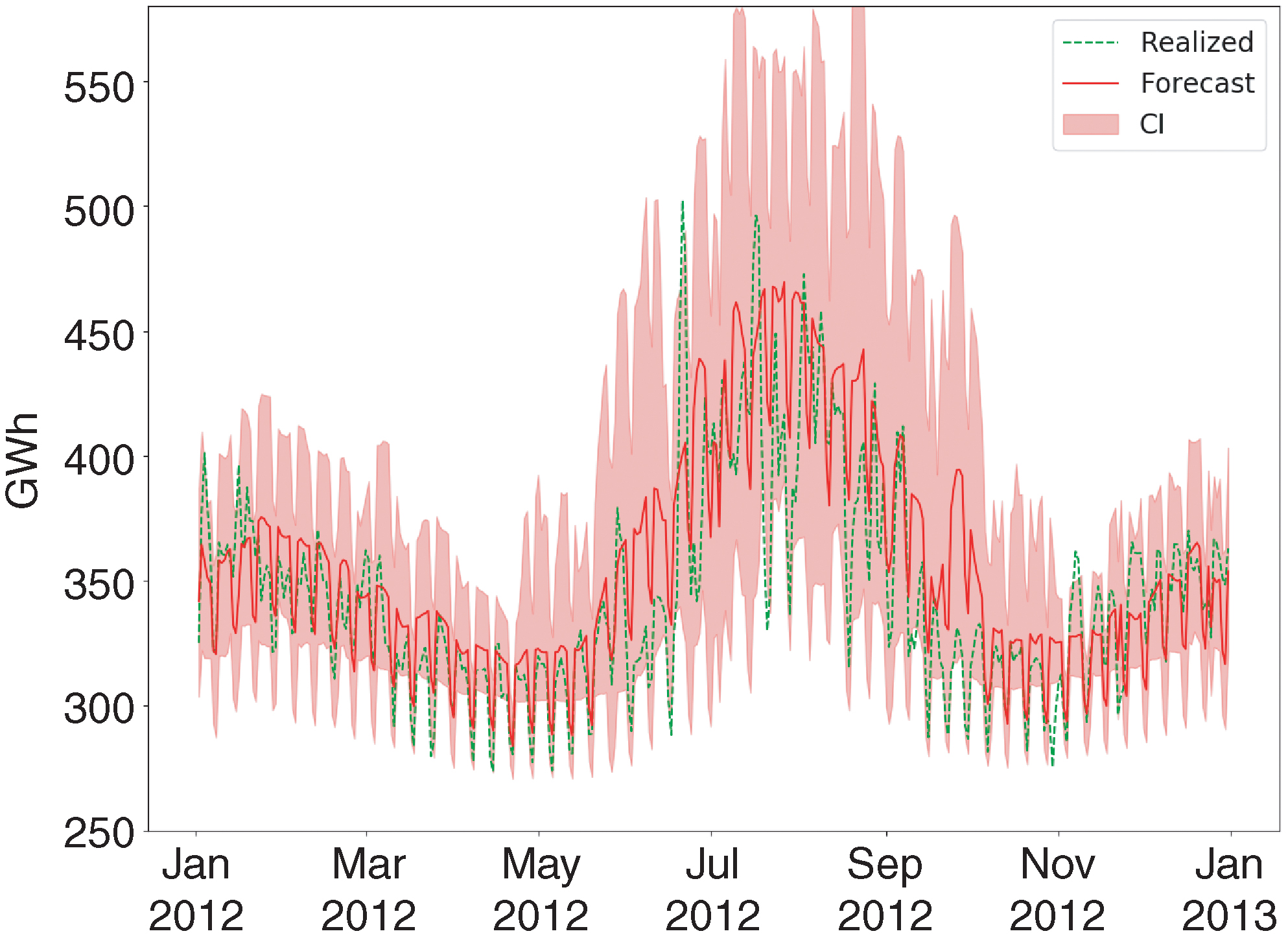
Second, Figure 12 shows the NAX power consumption middle-term ex ante density prediction. As in Figure 9 for the ex post case, the solid red line indicates the point forecast, while the shaded area indicates the 95% CI; the dashed green line shows the power consumption realized on the test set. As expected, our results are less accurate than those for the ex post prediction in terms of both the point forecast and the range of the CI because we consider the error in temperature forecasts. Despite this, the seasonality in both the volatility and the point forecast is preserved, and the reliability of the CI remains high (realized consumption falls within the 95% CI on all but 22 days, 94.0% of cases).

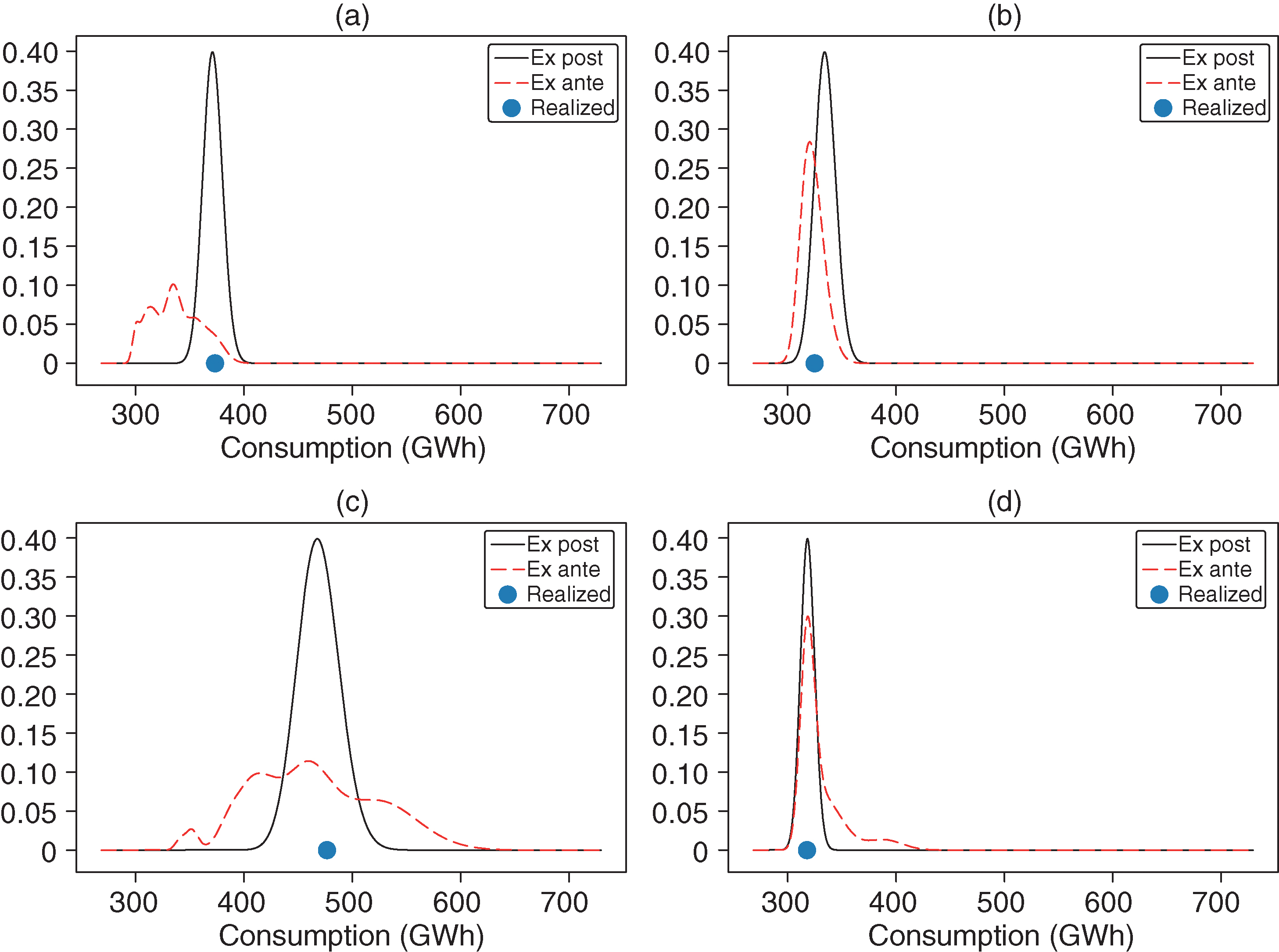
To show the forecasting density change after introducing the error in temperatures, in Figure 13 we analyze four days (in winter, spring, summer and fall). In all cases, we observe a wider distribution in the ex ante forecast, and the realized consumption falls within the densities. Note that the ex ante distributions are always wider, particularly in summer and winter, while during spring and fall the two forecasts look quite close.

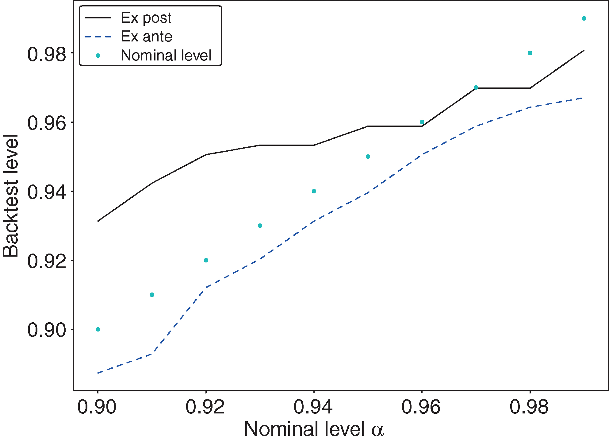
Finally, we can backtest the CI, counting the fraction of days on which the realized power consumption falls outside a confidence level $\alpha$ for the predicted density (violations) and comparing this with the nominal values, equal to $1-\alpha$. In Figure 14, we can observe that both ex post and ex ante CIs are close to the nominal values. We must take into account the sharpness of the ex post CI compared with the ex ante CI (cf, Figures 9 and 12).

In this section, we have presented the ex ante density forecast. As expected, we observed an increase in the point forecasting error and a widening of the CI with respect to the ex post case. However, the density forecast remains sufficiently accurate and the seasonality structure (both in the point forecasting and in the volatility) is preserved, showing the robustness of the NAX density forecasts.

6 Concluding remarks

In this paper, we introduced the NAX model for middle-term density forecasting of power consumption, a hybrid model that combines the advantages of classical univariate time series analysis and a shallow NN.

The main contributions of this paper are threefold. First, the NN architecture (described in Figure 4) is new to the literature: it is designed to obtain both a density forecast and the autoregressive feature observed in the consumption time series. Second, we showed that NAX achieves an excellent middle-term forecast of power consumption using only weather data. We achieve an ex post MAPE of less than 2% on the testing set (see Table 4), 20% better than GPX in relative terms, and the realized power consumption is forecast with great accuracy (see Figure 9). Third, we valued the density forecast via some sharpness and reliability measures, showing the quality of the results achieved (see Figures 10 and 11). The robustness of NAX performance over time, in terms of both point (MAPE and RMSE) and density (APL) forecasting, was tested from 2013 to 2016 (see Table 6). We also showed an ex ante middle-term density forecast as an application of our proposed technique.

These results show that our proposed model can accurately capture the relationship between weather conditions and power consumption distribution in a sharp and reliable way, even considering short time series with only a few years of daily training window data.

Declaration of interest

The authors report no conflicts of interest. The authors alone are responsible for the content and writing of the paper.

Acknowledgements

We thank Y. Chen, M. De Prato, S. Grassi, J. Turiel and all the participants at the 2020 AI, Financial Automation and Market Risk Workshop. This work was supported by FinTech Ho2020.eu, “A FINancial supervision and TECHnology compliance training programme”.

References

• Baviera, R., and Messuti, G. (2020). Daily middle-term probabilistic forecasting of power consumption in North-East England. Preprint (arXiv:2005.13005).
• Benth, F. E., Benth, J. S., and Koekebakker, S. (2008). Stochastic Modelling of Electricity and Related Markets. World Scientific, Singapore (https://doi.org/10.1142/6811).
• Box, G. E., Jenkins, G. M., Reinsel, G. C., and Ljung, G. M. (2015). Time Series Analysis: Forecasting and Control. Wiley.
• Christoffersen, P. F. (1998). Evaluating interval forecasts. International Economic Review 39(4), 841–862 (https://doi.org/10.2307/2527341).
• Fan, S., and Chen, L. (2006). Short-term load forecasting based on an adaptive hybrid method. IEEE Transactions on Power Systems 21(1), 392–401 (https://doi.org/10.1109/TPWRS.2005.860944).
• Felder, M., Kaifel, A., and Graves, A. (2010). Wind power prediction using mixture density recurrent neural networks. In Proceedings of European Wind Energy Conference and Exhibition, pp. 3417–3424. WindEurope, Brussels.
• Goude, Y., Nedellec, R., and Kong, N. (2013). Local short and middle term electricity load forecasting with semi-parametric additive models. IEEE Transactions on Smart Grid 5(1), 440–446 (https://doi.org/10.1109/TSG.2013.2278425).
• Hong, T., and Fan, S. (2016). Probabilistic electric load forecasting: a tutorial review. International Journal of Forecasting 32(3), 914–938 (https://doi.org/10.1016/j.ijforecast.2015.11.011).
• Hong, T., Pinson, P., Fan, S., Zareipour, H., Troccoli, A., and Hyndman, R. J. (2016). Probabilistic energy forecasting: global energy forecasting competition 2014 and beyond. International Journal of Forecasting 32(3), 896–913 (https://doi.org/10.1016/j.ijforecast.2016.02.001).
• Hyndman, R., and Fan, S. (2010). Density forecasting for long-term peak electricity demand. IEEE Transactions on Power Systems 25(2), 1142–1153 (https://doi.org/10.1109/TPWRS.2009.2036017).
• Kong, W., Dong, Z. Y., Jia, Y., Hill, D. J., Xu, Y., and Zhang, Y. (2017). Short-term residential load forecasting based on LSTM recurrent neural network. IEEE Transactions on Smart Grid 10(1), 841–851 (https://doi.org/10.1109/TSG.2017.2753802).
• Kupiec, P. (1995). Techniques for verifying the accuracy of risk measurement models. Journal of Derivatives 3(2), 73–84 (https://doi.org/10.3905/jod.1995.407942).
• LeCun, Y., Bengio, Y., and Hinton, G. (2015). Deep learning. Nature 521(7553), 436–444 (https://doi.org/10.1038/nature14539).
• Meng, K., Dong, Z. Y., and Wong, K. P. (2009). Self-adaptive radial basis function neural network for short-term electricity price forecasting. IET Generation, Transmission Distribution 3(4), 325–335 (https://doi.org/10.1049/iet-gtd.2008.0328).
• Nikolaev, N., Tino, P., and Smirnov, E. (2013). Time-dependent series variance learning with recurrent mixture density networks. Neurocomputing 122, 501–512 (https://doi.org/10.1016/j.neucom.2013.05.014).
• Nowotarski, J., and Weron, R. (2018). Recent advances in electricity price forecasting: a review of probabilistic forecasting. Renewable and Sustainable Energy Reviews 81, 1548–1568 (https://doi.org/10.1016/j.rser.2017.05.234).
• Ormoneit, D., and Neuneier, R. (1996). Experiments in predicting the German stock index DAX with density estimating neural networks. In IEEE/IAFE 1996 Conference on Computational Intelligence for Financial Engineering (CIFEr), pp. 66–71. IEEE Press, Piscataway, NJ (https://doi.org/10.1109/CIFER.1996.501825).
• Patro, S., and Sahu, K. K. (2015). Normalization: a preprocessing stage. International Advanced Research Journal in Science, Engineering and Technology 2(3), 20–22 (https://doi.org/10.17148/IARJSET.2015.2305).
• Rasmussen, C., and Williams, C. (2006). Gaussian Processes for Machine Learning. Adaptive Computation and Machine Learning. MIT Press, Cambridge, MA (https://doi.org/10.7551/mitpress/3206.001.0001).
• Ripley, B. D. (2007). Pattern Recognition and Neural Networks. Cambridge University Press.
• Rodrigues, F., Cardeira, C., and Calado, J. M. F. (2014). The daily and hourly energy consumption and load forecasting using artificial neural network method: a case study using a set of 93 households in Portugal. Energy Procedia 62, 220–229 (https://doi.org/10.1016/j.egypro.2014.12.383).
• Shi, H., Xu, M., and Li, R. (2018). Deep learning for household load forecasting: a novel pooling deep RNN. IEEE Transactions on Smart Grid 9(5), 5271–5280 (https://doi.org/10.1109/TSG.2017.2686012).
• Vossen, J., Feron, B., and Monti, A. (2018). Probabilistic forecasting of household electrical load using artificial neural networks. In 2018 IEEE International Conference on Probabilistic Methods Applied to Power Systems, pp. 1–6. IEEE Press, Piscataway, NJ (https://doi.org/10.1109/PMAPS.2018.8440559).

Download PDF

• Keywords
• Electric utility
• Energy markets
• Original research
• Machine learning
• Neural networks
• Forecasting
• More
  Less