Numerical solution of the Hamilton–Jacobi–Bellman formulation for continuous-time mean–variance asset allocation under stochastic volatility

K Ma and P. A. Forsyth

Abstract

ABSTRACT

We present efficient partial differential equation (PDE) methods for continuous-time mean-variance portfolio allocation problems when the underlying risky asset follows a stochastic volatility process. The standard formulation for mean-variance optimal portfolio allocation problems gives rise to a two-dimensional nonlinear Hamilton–Jacobi–Bellman (HJB) PDE. We use a wide stencil method based on a local coordinate rotation to construct a monotone scheme. Further, by using a semi-Lagrangian timestepping method to discretize the drift term, along with an improved linear interpolation method, accurate efficient frontiers are constructed. This scheme can be shown to be convergent to the viscosity solution of the HJB equation, and the correctness of the proposed numerical framework is verified by numerical examples. We also discuss the effects on the efficient frontier of the stochastic volatility model parameters.

Download PDF

Introduction

1 Introduction

Consider the following prototypical asset allocation problem: an investor can choose to invest in a risk-free bond, or a risky asset, and can dynamically allocate wealth between the two assets, to achieve a predetermined criteria for the portfolio over a long time horizon. In the continuous-time mean–variance approach, risk is quantified by variance, so investors aim to maximize the expected return of their portfolios, given a risk level. Alternatively, they aim to minimize the risk level, given an expected return. As a result, mean–variance strategies are appealing due to their intuitive nature, since the results can be easily interpreted in terms of the trade-off between the risk and the expected return.

In the case where the asset follows a geometric Brownian motion (GBM), there is considerable literature on the topic (Li and Ng 2000; Bielecki et al 2005; Zhou and Li 2000; Wang and Forsyth 2010). The multi-period optimal strategy adopted in these papers is of pre-commitment type, which is not time consistent, as noted in Bjork and Murgoci (2010) and Basak and Chabakauri (2010). A comparison between time-consistent and pre-commitment strategies for continuous-time mean–variance optimization is given in Wang and Forsyth (2012). We note that since a time-consistent strategy can be constructed from a pre-commitment policy by adding a constraint (Wang and Forsyth 2012), the time-consistent strategy is suboptimal compared with the pre-commitment policy, ie, it is costly to enforce time consistency. In addition, it has been shown in Vigna (2014) that pre-commitment strategies can also be viewed as a target-based optimization, which involves minimizing a quadratic loss function. It is suggested in Vigna (2014) that this is intuitive, adaptable to investor preferences and also mean–variance efficient.

Most previous literature on pre-commitment mean–variance optimal asset allocation has been based on analytic techniques (Li and Ng 2000; Zhou and Li 2000; Bielecki et al 2005; Zhao and Ziemba 2000; Nguyen and Portait 2002). These papers have primarily employed martingale methods (Bielecki et al 2005; Zhao and Ziemba 2000; Nguyen and Portait 2002) or tractable auxiliary problems (Li and Ng 2000; Zhou and Li 2000). However, in general, if realistic constraints on portfolio selection are imposed, eg, no trading if insolvent and a maximum leverage constraint, then a fully numerical approach is required. As shown in Wang and Forsyth (2010), in the case where the risky asset follows a GBM, realistic portfolio constraints have a significant effect on the efficient frontier.

Another modeling deficiency in previous work on pre-commitment mean–variance optimal asset allocation is the common assumption that the risky asset follows a GBM. However, there is strong empirical evidence that asset return volatility is serially correlated, shocks to volatility are negatively correlated with asset returns and the conditional variance of asset returns is not constant over time. As a result, it is highly desirable to describe the risky asset with a stochastic volatility model. In this case, the standard formulation of mean–variance optimal asset allocation problems gives rise to a two-dimensional nonlinear Hamilton–Jacobi–Bellman (HJB) PDE. The objective of this paper is to develop a numerical method for the pre-commitment mean–variance portfolio selection problem when the underlying risky asset follows a stochastic volatility model.

The major contributions of the paper are the following.

• •

  We develop a fully implicit, consistent, unconditionally monotone numerical scheme for the HJB equation, which arises in the embedding formulation (Zhou and Li 2000; Li and Ng 2000) of the pre-commitment mean–variance problem under our model setup. The main difficulty in designing a discretization scheme is developing a monotone approximation of the cross-derivative term in the PDE. We use the wide stencil method (Debrabant and Jakobsen 2013; Ma and Forsyth 2014) to deal with this difficulty.

• •

  We construct accurate efficient frontiers by using a semi-Lagrangian time-stepping method to handle the drift term and an improved method of linear interpolation at the foot of the characteristic in the semi-Lagrangian discretization. In particular, the improved interpolation method uses the exact solution value at a single point, dramatically increasing the accuracy of the numerical results. Any type of constraint can be applied to the investment policy.

• •

  We prove that the scheme developed in this paper converges to the viscosity solution of the nonlinear HJB value equation.

• •

  In order to trace out the efficient frontier solution of our problem, we use two techniques: the PDE method and the hybrid (PDE–Monte Carlo) method (Tse et al 2013). We also demonstrate that the hybrid method is superior to the PDE method.

• •

  We carry out several numerical experiments, and illustrate the convergence of the numerical scheme as well as the effect of modeling parameters on efficient frontiers.

The remainder of this paper is organized as follows. Section 2 describes the underlying processes and the embedding framework, and gives a formulation of an associated HJB equation and a linear PDE. In Section 3, we present the discretization of the HJB equation. In Section 4, we highlight some important implementation details of the numerical method. Numerical results are presented and discussed in Section 5.

2 Mathematical formulation

Suppose there are two assets in the market: one is a risk-free bond, and the other is a risky equity index. The dynamics of the risk-free bond $B$ follows

$$\mathrm{d}B(t)=rB(t)\mathrm{d}t,$$

(2.1)

and an equity index $S$ follows Heston’s model (Heston 1993) under the real probability measure

$$\frac{\mathrm{d}S(t)}{S(t)}=(r+\xi V(t))\mathrm{d}t+\sqrt{V(t)}\mathrm{d}{Z}_1,$$

(2.2)

where the variance of the index, $V(t)$, follows a mean-reverting square-root process (Cox et al 1985):

$$\mathrm{d}V(t)=\kappa (\theta -V(t))\mathrm{d}t+\sigma \sqrt{V(t)}\mathrm{d}{Z}_2,$$

(2.3)

with $\mathrm{d}{Z}_1$, $\mathrm{d}{Z}_2$ being increments of Wiener processes. The instantaneous correlation between $Z_1$ and $Z_2$ is $\mathrm{d}{Z}_1\mathrm{d}{Z}_2=\rho \mathrm{d}t$. The market price of volatility risk is $\xi V(t)$, which generates a risk premium proportional to $V(t)$. This assumption for the risk premium is based on Breeden’s consumption-based model (Breeden 1979), and it originates from Heston (1993). Therefore, under this setup, the market is incomplete, as trading in the risky asset and the bond cannot perfectly hedge the changes in the stochastic investment opportunity set.

An investor in this market is endowed at time zero with an initial wealth of $w_0$, and they can continuously and dynamically alter the proportion of wealth invested in each asset. In addition, let $W(t)=S(t)+B(t)$ denote the wealth at time $t$, and let $p$ denote the proportion of this wealth invested in the risky asset $S(t)$; consequently, $(1-p)$ denotes the fraction of wealth invested in the risk-free bond $B(t)$. The allocation strategy is a function of the current state, ie, $p(\cdot ):(W(t),V(t),t)\to p=p(W(t),V(t),t)$. Note that in using the shorthand notations $p(\cdot )$ for the mapping, $p$ for the value $p=p(W(t),V(t),t)$, and the dependence on the current state is implicit. From (2.1) and (2.2), we see that the investor’s wealth process follows

$$\mathrm{d}W(t)=(r+p\xi V(t))W(t)\mathrm{d}t+p\sqrt{V}W(t)\mathrm{d}{Z}_1.$$

(2.4)

2.1 Efficient frontiers and embedding methods

We assume here that the investor is guided by a pre-commitment mean–variance objective based on the final wealth $W(T)$. The pre-commitment mean–variance problem and its variations have been intensively studied in the literature (Li and Ng 2000; Zhou and Li 2000; Bielecki et al 2005; Zhao and Ziemba 2000; Nguyen and Portait 2002). To the best of our knowledge, there is no explicit closed-form solution for the pre-commitment mean–variance problem when the risky asset follows a stochastic volatility process along with leverage constraints.

To simplify our notation, we define $x=(w,v)=(W(t),V(t))$ for a state space. Let $E_{p(\cdot )}^{x,t}[W(T)]$ and ${\mathrm{Var}}_{p(\cdot )}^{x,t}[W(T)]$ denote the expectation and variance of the terminal wealth conditional on the state $(x,t)$ and the control $p(\cdot )$. Given a risk level ${\mathrm{Var}}_{p(\cdot )}^{x,t}[W(T)]$, an investor desires their expected terminal wealth $E_{p(\cdot )}^{x,t}[W(T)]$ to be as large as possible. Equivalently, given an expected terminal wealth $E_{p(\cdot )}^{x,t}[W(T)]$, they wish the risk ${\mathrm{Var}}_{p(\cdot )}^{x,t}[W(T)]$ to be as small as possible. That is, they desire to find controls $p(\cdot )$ that generate Pareto optimal points. For notational simplicity, let $E_{p(\cdot )}^{x,t}[W(T)]=ℰ$ and ${\mathrm{Var}}_{p(\cdot )}^{x,t}[W(T)]=?$. The problem is rigorously formulated as follows.

Define the achievable mean–variance objective set as

$$?=\{(?,ℰ):p\in ?\},$$

(2.5)

where $?$ is the set of admissible strategies, and denote the closure of $?$ by $\overline{?}$.

Definition 2.1.

A point $(?,ℰ)\in ?$ is Pareto mean–variance optimal if there exists no admissible strategy $\overline{p}\in ?$ such that

$${\mathrm{Var}}_{\overline{p}}^{x,t}\{W(T)\}\le ?,E_{\overline{p}}^{x,t}\{W(T)\}\ge ℰ,$$

(2.6)

where at least one of the inequalities in the equation is strict. We denote by $?$ the set of Pareto mean–variance optimal points. Note that $?\subseteq \overline{?}$.

Although the above definition is intuitive, determining the points in $?$ requires the solution of a multi-objective optimization problem, involving two conflicting criteria. A standard scalarization method can be used to combine the two criteria into an optimization problem with a single objective. In particular, for each point $(?,ℰ)\in \overline{?}$, and for an arbitrary scalar $\lambda >0$, we define the set of points ${?}_{P(\lambda )}$ to be

$${?}_{P(\lambda )}=\{(?,ℰ)\in \overline{?}:\underset{({?}_{*},{ℰ}_{*})\in ?}{inf}(\lambda {?}_{*}-{ℰ}_{*})\},$$

(2.7)

from which a point on the efficient frontier can be derived. The set of points on the efficient frontier is then defined as

$${?}_P=\bigcup _{\lambda >0}{?}_{P(\lambda )}.$$

(2.8)

Note that there is a difference between the set of all Pareto mean–variance optimal points $?$ (see Definition 2.1) and the efficient frontier ${?}_P$ (2.8) (Tse et al 2014). In general,

$$?\subseteq {?}_P,$$

but the converse may not hold if the achievable mean–variance objective set $?$ (2.5) is not convex. In this paper, we restrict our attention to constructing ${?}_P$ (2.8).

Due to the presence of the variance term ${\mathrm{Var}}_{p(\cdot )}^{x,t}[W(T)]$ in (2.7), a dynamic programming principle cannot be directly applied to solve this problem. To overcome this difficulty, we make use of the main result in Li and Ng (2000), Zhou and Li (2000) and Tse et al (2014), which essentially involves the embedding technique. This result is summarized in Theorem 2.3.

Assumption 2.2.

We assume that $\mathrm{Y}$ is a non-empty subset of $\mathrm{\{}\mathrm{(}\mathrm{V}\mathrm{,}\mathrm{E}\mathrm{)}\mathrm{\in }{\mathrm{R}}^{\mathrm{2}}\mathrm{:}\mathrm{V}\mathrm{>}\mathrm{0}\mathrm{\}}$ and that there exists a positive scalarization parameter ${\lambda }_E\mathrm{>}\mathrm{0}$ such that ${\mathrm{Y}}_{P\mathit{}\mathrm{(}{\lambda }_E\mathrm{)}}\mathrm{\ne }\mathrm{\varnothing }$.

Theorem 2.3.

The embedded mean–variance objective set ${\mathrm{Y}}_Q$ is defined by

(2.9)

where

$${?}_{Q(\gamma )}=\{({?}_{*},{ℰ}_{*})\in \overline{?}:{?}_{*}+{ℰ}_{*}^2-\gamma {ℰ}_{*}=\underset{(?,ℰ)\in ?}{inf}(?+{ℰ}^2-\gamma ℰ)\}.$$

(2.10)

If Assumption 2.2 holds and $\lambda \mathrm{>}{\lambda }_E$, then ${\mathrm{Y}}_{P\mathit{}\mathrm{(}\lambda \mathrm{)}}\mathrm{\ne }\mathrm{\varnothing }$. Assume $\mathrm{(}{\mathrm{V}}_{\mathrm{0}}\mathrm{,}{\mathrm{E}}_{\mathrm{0}}\mathrm{)}\mathrm{\in }{\mathrm{Y}}_{P\mathit{}\mathrm{(}\lambda \mathrm{)}}$. Then, if

$$\lambda {?}_0-{ℰ}_0=\underset{(?,ℰ)\in ?}{inf}(\lambda ?-ℰ),$$

(2.11)

then

$${?}_0+{ℰ}_0^2-\gamma {ℰ}_0=\underset{(?,ℰ)\in ?}{inf}(?+{ℰ}^2-\gamma ℰ),\mathit{\text{ie, }}({?}_0,{ℰ}_0)\in {?}_{Q(\gamma )},$$

(2.12)

where $\gamma \mathrm{=}\mathrm{(}\mathrm{1}\mathrm{/}\lambda \mathrm{)}\mathrm{+}\mathrm{2}\mathit{}{\mathrm{E}}_{\mathrm{0}}$. Consequently, ${\mathrm{Y}}_P\mathrm{\subseteq }{\mathrm{Y}}_Q$.

Proof.

See details in Li and Ng (2000), Zhou and Li (2000) and Dang et al (2016). ∎

Theorem 2.3 states that the mean and variance $(?,ℰ)$ of $W(T)$ are embedded in a scalarization optimization problem, with the objective function being $?+{ℰ}^2-\gamma ℰ$. Noting that

	$?+{ℰ}^2-\gamma ℰ$	$=E_{p(\cdot )}^{x,t}[W^2(T)]-{(E_{p(\cdot )}^{x,t}[W(T)])}^2+{(E_{p(\cdot )}^{x,t}[W(T)])}^2-\gamma E_{p(\cdot )}^{x,t}[W(T)]$
		$=E_{p(\cdot )}^{x,t}[W^2(T)-\gamma W(T)]$
		$=E_{p(\cdot )}^{x,t}[{(W(T)-\frac{1}{2}\gamma )}^2]+\frac{1}{4}{\gamma }^2,$		(2.13)

and that we can ignore the constant $\frac{1}{4}{\gamma }^2$ term for the purposes of minimization, we then define the value function

$$?(x,t)=\underset{p(\cdot )\in ?}{inf}{E}_{p(\cdot )}^{x,t}[{(W(T)-\frac{1}{2}\gamma )}^2].$$

(2.14)

Theorem 2.3 implies that there exists a $\gamma$ such that, for a given positive $\lambda$, a control $p^{*}$ that minimizes (2.7) also minimizes (2.14). Dynamic programming can then be directly applied to (2.14) to determine the optimal control $p^{*}(\cdot )$.

The procedure for determining the points on the efficient frontier is as follows. For a given value of $\gamma$, the optimal strategy $p^{*}$ is determined by solving for the value function problem (2.14). Once this optimal policy $p^{*}(\cdot )$ is known, it is then straightforward to determine a point $({\mathrm{Var}}_{p^{*}(\cdot )}^{x,t}[W(T)],E_{p^{*}(\cdot )}^{x,t}[W(T)])$ on the frontier. Varying $\gamma$ traces out a curve in the $(?,ℰ)$ plane (see details in Section 4.2). Consequently, the numerical challenge is to solve for the value function (2.14). More precisely, the above procedure for constructing the efficient frontier generates points that are in the set ${?}_Q$. As pointed out in Tse et al (2014), the set ${?}_Q$ may contain spurious points, ie, points that are not in ${?}_P$. For example, when the original problem is nonconvex, spurious points can be generated. An algorithm for removing spurious points is discussed in Tse et al (2014). The set of points in ${?}_Q$ with the spurious points removed generates all points in ${?}_P$. Dang et al (2016) also discusses the convergence of finitely sampled $\gamma$ to the efficient frontier.

Remark 2.4 (Range of $\gamma$).

As noted in Dang et al (2016), a solution to (2.10) generally exists for all $\gamma \in (-\mathrm{\infty },+\mathrm{\infty })$. However, we know from the above discussion that some of these solutions may be spurious. In some cases, we can use financial reasoning to reduce the range of $\gamma$ so that obvious spurious points are eliminated. We discuss this further in Section 4.2.1.

2.2 The value function problem

Following standard arguments, the value function $?(w,v,\tau )$, $\tau =T-t$ (2.14) is the viscosity solution of the HJB equation

$${?}_{\tau }=\underset{p\in ?}{inf}\{(r+p\xi v)w{?}_w+\kappa (\theta -v){?}_v+\frac{1}{2}{(p\sqrt{v}w)}^2{?}_{ww}+p\rho \sigma \sqrt{v}w{?}_{wv}+\frac{1}{2}{\sigma }^{2}v{?}_{vv}\},$$

(2.15)

on the domain $(w,v,\tau )\in [0,+\mathrm{\infty }]\times [0,+\mathrm{\infty }]\times [0,T]$, and with the terminal condition

$$?(w,v,0)={(w-\frac{1}{2}\gamma )}^2.$$

(2.16)

Remark 2.5.

In one of our numerical tests, we allow $p$ to become unbounded, which may occur when $w\to 0$ (Wang and Forsyth 2010). However, although $p\to \mathrm{\infty }$ as $w\to 0$, we must have $(pw)\to 0$ as $w\to 0$, ie, the amount invested in the risky asset converges to zero as $w\to 0$. This is required in order to ensure that the no-bankruptcy boundary condition is satisfied (Wang and Forsyth 2010). As a result, we can then formally eliminate the problem with unbounded control by using $q=pw$ as the control, and assume $q$ remains bounded (see details in Wang and Forsyth (2010)).

2.3 The expected wealth problem

2.3.1 The PDE formulation

Given the solution for the value function (2.14), with the optimal control $p^{*}(\cdot )$, we then need to determine the expected value $E_{p^{*}(\cdot )}^{x,t}[W(T)]$, denoted as

$$ℰ(w,v,t)=E_{p^{*}(\cdot )}^{x,t}[W(T)].$$

(2.17)

Then, $ℰ(w,v,\tau )$, $\tau =T-t$ is given from the solution to the following linear PDE:

$${ℰ}_{\tau }=(r+p^{*}\xi v)w{ℰ}_w+\kappa (\theta -v){ℰ}_v+\frac{1}{2}{(p^{*}\sqrt{v}w)}^2{ℰ}_{ww}+p^{*}\rho \sigma \sqrt{v}w{ℰ}_{wv}+\frac{1}{2}{\sigma }^{2}v{ℰ}_{vv},$$

(2.18)

with the initial condition $ℰ(w,v,0)=w$, where $p^{*}$ is obtained from the solution of the HJB equation (2.15).

2.3.2 The hybrid (PDE–Monte Carlo) method

Alternatively, given the stored control $p^{*}(\cdot )$ determined from the solution of (2.15), we can directly estimate $({\mathrm{Var}}_{p^{*}(\cdot )}^{x,t}[W(T)],E_{p^{*}(\cdot )}^{x,t}[W(T)])$ by using a Monte Carlo method, based on solving the stochastic differential equations (SDEs) (2.3) and (2.4). The details of the SDE discretization are given in Section 4.2. This hybrid (PDE–Monte Carlo) method was originally proposed in Tse et al (2013).

2.4 Allowable portfolios

In order to obtain analytical solutions, many previous papers typically make assumptions that allow for the possibility of unbounded borrowing and bankruptcy. Moreover, these models assume a bankrupt investor can still keep on trading. The ability to continue trading even though the value of an investor’s wealth is negative is highly unrealistic. In this paper, we enforce the condition that the wealth value remains in the solvency regions by applying certain boundary conditions to the HJB equation (Wang and Forsyth 2008). Thus, bankruptcy is prohibited, ie,

$$w\in [0,+\mathrm{\infty }).$$

We will also assume that there is a leverage constraint, ie, the investor must select an asset allocation satisfying

which can be interpreted as the maximum leverage condition, and $p_{\max }$ is a known positive constant with typical value in $[1.0,2.0]$. Thus, the control set

$$p\in ?=[0,p_{\max }].$$

Note that when the risk premium $\xi$ (2.2) is positive, as in our case, it is not optimal to short the risky asset, since we have only a single risky asset in our portfolio. In some circumstances, it may be optimal to short the risky asset. This will be discussed in Section 3.1.3.

3 Numerical discretization of the Hamilton–Jacobi–Bellman equation

3.1 Localization

We will assume that the discretization is posed on a bounded domain for computational purposes. The discretization is applied to the localized finite region $(w,v)\in [0,w_{\max }]\times [0,v_{\max }]$. Asymptotic boundary conditions will be imposed at $w=w_{\max }$ and $v=v_{\max }$, which are compatible with a monotone numerical scheme.

3.1.1 The localization of $V$

The proper boundary on $v=0$ needs to be specified to be compatible with the corresponding SDE (2.3), which has a unique solution (Feller 1951). If $2\kappa \theta \ge {\sigma }^2$, the so-called Feller condition holds, and $v=0$ is unattainable. If the Feller condition is violated, , then $v=0$ is an attainable boundary but is strongly reflecting (Feller 1951). The appropriate boundary condition can be obtained by setting $v=0$ into (2.15). That is,

$${?}_{\tau }=rw{?}_w+\kappa \theta {?}_v,$$

(3.1)

and the equation degenerates to a linear PDE. On the lower boundary $v=0$, the variance and the risk premium vanish, according to (2.4), so that the wealth return is always the risk-free rate $r$. The control value $p$ vanishes in the degenerate equation (3.1), and we can simply define $p^{*}(w,v=0,t)\equiv 0$, which we need in the estimation of $({\mathrm{Var}}_{p^{*}(\cdot )}^{x,t}[W(T)],E_{p^{*}(\cdot )}^{x,t}[W(T)])$ using the Monte Carlo simulation. In this case, since the equity asset has zero volatility with drift rate $r$, the distinction between the equity asset and risk-free asset is meaningless.

The validity of this boundary condition is intuitively justified by the fact that the solution to the SDE for $v$ is unique, such that the behavior of $v$ at the boundary $v=0$ is determined by the SDE itself, and, hence, the boundary condition is determined by setting $v=0$ in (2.15). A formal proof that this boundary condition is correct is given in Ekström and Tysk (2010). If the boundary at $v=0$ is attainable, then this boundary behavior serves as a boundary condition and guarantees uniqueness in the appropriate function spaces. However, if the boundary is non-attainable, then the boundary behavior is not needed to guarantee uniqueness, but it is nevertheless very useful in a numerical scheme.

On the upper boundary $v=v_{\max }$, ${?}_v$ is set to zero. Thus, the boundary condition on $v_{\max }$ is set to

$${?}_{\tau }=\underset{p\in ?}{inf}\{(r+p\xi v)w{?}_w+\frac{1}{2}{(p\sqrt{v}w)}^2{?}_{ww}\}.$$

(3.2)

The optimal control $p^{*}$ at $v=v_{\max }$ is determined by solving (3.2). This boundary condition can be justified by noting that, as $v\to \mathrm{\infty }$, the diffusion term in the $w$ direction in (2.15) becomes large. In addition, the initial condition (2.16) is independent of $v$. As a result, we expect that

$$?\approx C^{\prime }w+C^{\prime \prime },v\to \mathrm{\infty },$$

where $C^{\prime }$ and $C^{\prime \prime }$ are constants, and, hence, ${?}_v\approx 0$ at $v=v_{\max }$.

3.1.2 The localization for $W$

We prohibit the possibility of bankruptcy by requiring ${lim}_{w\to 0}(pw)=0$ (Wang and Forsyth 2010), so, on $w=0$, (2.15) reduces to

$${?}_{\tau }=\kappa (\theta -v){?}_v+{\sigma }^{2}v{?}_{vv}.$$

(3.3)

When $w\to +\mathrm{\infty }$, we assume that the asymptotic form of the exact solution is

$$?(w\to +\mathrm{\infty },v,\tau )=\overline{?}(w)=H_2(\tau )w^2+H_1(\tau )w+H_0(\tau );$$

(3.4)

we make the assumption that $p^{*}(w_{\max },v,0)$ at $w=w_{\max }$ is set to zero. That is, once the investor’s wealth is very large, they prefer the risk-free asset. This can be justified from the arguments in Cui et al (2012) and Dang and Forsyth (2014a).

Substituting form (3.4) into PDE (2.15) and setting $p=0$, we obtain

$${(H_0)}_{\tau }=0,{(H_1)}_{\tau }=r{H}_1,{(H_2)}_{\tau }=2r{H}_2.$$

Initial conditions are determined from (2.16) and (3.4):

$$H_0(0)=\frac{1}{4}{\gamma }^2,H_1(0)=-2\gamma ,H_2(0)=1.$$

3.1.3 Alternative localization for $w$

$?(w,v,\tau )$ is the viscosity solution of the HJB equation (2.15). Recall that the initial condition for problem (2.14) is

$$?(w,v,0)={(W(T)-\frac{1}{2}\gamma )}^2.$$

For a fixed gamma, we define the discounted optimal embedded terminal wealth at time $t$, denoted by $W_{\text{opt}}(t)$, as

$$W_{\text{opt}}(t)=\frac{1}{2}\gamma {\mathrm{e}}^{-r(T-t)}.$$

(3.5)

It is easy to verify that $W_{\text{opt}}(t)$ is a global minimum state of the value function $?(w,v,t)$. Consider the state $(W_{\text{opt}}(t),v)$, $t\in [0,T]$, and the optimal strategy $p^{*}(\cdot )$ such that $p^{*}(w,v,?)\equiv 0$, $?>t$. Under $p^{*}(\cdot )$, the wealth is all invested in the risk-free bond without further rebalancing from time $t$. As a result, the wealth will accumulate to $W(T)=\frac{1}{2}\gamma$ with certainty, ie, the optimal embedded terminal wealth $\frac{1}{2}\gamma$ is achievable. By (2.14), we have

$$?(W_{\text{opt}}(t),v,t)=\underset{p(\cdot )\in ?}{inf}\{E_{p(\cdot )}^{x,t}[{(W(T)-\frac{1}{2}\gamma )}^2]\}=E_{p^{*}(\cdot )}^{x,t}[{(W(T)-\frac{1}{2}\gamma )}^2]=0.$$

(3.6)

Since the value function is the expectation of a nonnegative quantity, it can never be less than zero. Hence, the exact solution for the value function problem at the special point $W_{\text{opt}}(t)$ must be zero. This result holds for both the discrete and continuous rebalancing case. For the formal proof, we refer the reader to Dang and Forsyth (2014a).

Consequently, the point $w=\frac{1}{2}\gamma {\mathrm{e}}^{-r\tau }$ is a Dirichlet boundary $?(\frac{1}{2}\gamma {\mathrm{e}}^{-r\tau },v,\tau )=0$, and information for $w>\frac{1}{2}\gamma {\mathrm{e}}^{-r\tau }$ is not needed. In principle, we can restrict the domain to $0\le w\le \frac{1}{2}\gamma {\mathrm{e}}^{-r\tau }$. However, it is computationally convenient to restrict the size of the computational domain to be $0\le w\le \frac{1}{2}\gamma$, which avoids the issue of having a moving boundary, at a very small additional cost. Note that the optimal control will ensure that $?(\frac{1}{2}\gamma {\mathrm{e}}^{-r\tau },v,\tau )=0$ without any need to enforce this boundary condition. This will occur, as we assume continuous rebalancing. This effect, that $W(t)\le W_{\text{opt}}(t)$, is also discussed in Vigna (2014). It is interesting to note that, in the case of discrete rebalancing or jump diffusions, it is optimal to withdraw cash from the portfolio if it is ever observed that $W(t)>W_{\text{opt}}(t)$. However, Bauerle and Grether (2015) show that if the market is complete, then it is never optimal to withdraw cash from the portfolio. This is also discussed in Cui et al (2012) and Dang and Forsyth (2014a).

In the case of an incomplete market, such as discrete rebalancing or jump diffusions, if we do not allow the withdrawing of cash from the portfolio, then the investor has an incentive to lose money if $W(t)>W_{\text{opt}}(t)$, as pointed out in Cui et al (2012). In this rather perverse situation, it may be optimal to short the risky asset, so that the admissible set in this case would be $?=[p_{\min },p_{\max }]$, with .

We have verified, experimentally, that restricting the computational domain to $w\in [0,\frac{1}{2}\gamma ]$ gives the same results as the domain $w\in [0,w_{\max }]$, $w_{\max }\gg \frac{1}{2}\gamma$, with asymptotic boundary condition (3.4).

Remark 3.1 (Significance of $W(t)\le W_{\text{opt}}(t)$).

If we assume that initially (otherwise, the problem is trivial if we allow cash withdrawals), then the optimal control will ensure that $W(t)\le W_{\text{opt}}(t)$ for all $t$. Hence, continuous-time mean–variance optimization is “time consistent in efficiency” (Cui et al 2012). Another interpretation is that continuous-time mean–variance optimization is equivalent to minimizing the quadratic loss with respect to the wealth target $W_{\text{opt}}(T)$ (Vigna 2014).

Remark 3.2 (Significance of $W(T)\le \frac{1}{2}\gamma$).

From Remark 3.1, we have trivially that $W(T)\le \frac{1}{2}\gamma$; hence, from (2.14), the investor is never penalized for large gains, ie, the quadratic utility function (2.14) is always well behaved. Consequently, continuous-time mean–variance optimization is fundamentally different from its single-period counterpart.

3.2 Discretization

In the following section, we discretize (2.15) over a finite grid $N=N_1\times N_2$ in the space $(w,v)$. Define a set of nodes $\{w_1,w_2,\mathrm{\dots },w_{N_1}\}$ in the $w$ direction and $\{v_1,v_2,\mathrm{\dots },v_{N_2}\}$ in the $v$ direction. Denote the $n$th time step by ${\tau }^n=n\mathrm{\Delta }\tau$, $n=0,\mathrm{\dots },N_{\tau }$, with $N_{\tau }=T/\mathrm{\Delta }\tau$. Let ${?}_{i,j}^n$ be the approximate solution of (2.15) at $(w_i,v_j,{\tau }^n)$.

It will be convenient to define

	$\mathrm{\Delta }{w}_{\max }$	$=\underset{i}{\max }(w_{i+1}-w_i),$	$\mathrm{\Delta }{w}_{\min }$	$=\underset{i}{\min }(w_{i+1}-w_i),$
	$\mathrm{\Delta }{v}_{\max }$	$=\underset{i}{\max }(v_{i+1}-v_i),$	$\mathrm{\Delta }{v}_{\min }$	$=\underset{i}{\min }(v_{i+1}-v_i).$

We assume that there is a mesh discretization parameter $h$ such that

$$\mathrm{\Delta }{w}_{\max }=C_{1}h,\mathrm{\Delta }{w}_{\min }=C_{2}h,\mathrm{\Delta }{v}_{\max }=C_1^{\prime }h,\mathrm{\Delta }{v}_{\min }=C_2^{\prime }h,\mathrm{\Delta }\tau =C_{3}h,$$

(3.7)

where $C_1$, $C_2$, $C_1^{\prime }$, $C_2^{\prime }$, $C_3$ are constants independent of $h$.

In the following sections, we will give the details of the discretization for a reference node $(w_i,v_j)$, , .

3.2.1 The wide stencil

We need a monotone discretization scheme in order to guarantee convergence to the desired viscosity solution (Barles and Souganidis 1991). We remind the reader that seemingly reasonable non-monotone discretizations can converge to the incorrect solution (Pooley et al 2003). Due to the cross-derivative term in (2.15), however, a classic finite difference method cannot produce such a monotone scheme. Since the control appears in the cross-derivative term, it will not be possible (in general) to determine a grid spacing or global coordinate transformation that eliminates this term. We will adopt the wide stencil method developed in Ma and Forsyth (2014) to discretize the second derivative terms. Suppose we discretize (2.15) at grid node $(i,j)$ for a fixed control. For a fixed $p$, consider a virtual rotation of the local coordinate system clockwise by the angle ${\eta }_{i,j}$:

$${\eta }_{i,j}=\frac{1}{2}{\tan }^{-1}\left(\frac{2\rho p\sigma w_i{v}_j}{{(p\sqrt{v_j}{w}_i)}^2-{(\sigma \sqrt{v_j})}^2}\right).$$

(3.8)

That is, $(y_1,y_2)$ in the transformed coordinate system is obtained by using the following matrix multiplication:

(3.9)

We denote the rotation matrix in (3.9) as ${?}_{i,j}$. This rotation operation will result in a zero correlation in the diffusion tensor of the rotated system. Under this grid rotation, the second-order terms in (2.18) are, in the transformed coordinate system $(y_1,y_2)$,

$$a_{i,j}\frac{{\partial }^2?}{\partial y_1^2}+b_{i,j}\frac{{\partial }^2?}{\partial y_2^2},$$

(3.10)

where $?$ is the value function $?(y_1,y_2,\tau )$ in the transformed coordinate system, and

(3.11)

The diffusion tensor in (3.10) is diagonally dominant with no off-diagonal terms; consequently, a standard finite difference discretization for the second partial derivatives results in a monotone scheme. The rotation angle ${\eta }_{i,j}$ depends on the grid node and the control; therefore, it is impossible to rotate the global coordinate system by a constant angle and build a grid over the entire space $(y_1,y_2)$. The local coordinate system rotation is only used to construct a virtual grid, which overlays the original mesh. We have to approximate the values of $?$ on our virtual local grid using an interpolant ${?}_h?$ on the original mesh. To keep the numerical scheme monotone, ${?}_h$ must be a linear interpolation operator. Moreover, to keep the numerical scheme consistent, we need to use the points on our virtual grid, whose Euclidean distances are $O(\sqrt{h})$ from the central node, where $h$ is the mesh discretization parameter (3.7). This results in a wide stencil method, since the relative stencil length increases as the grid is refined ($\sqrt{h}/h\to +\mathrm{\infty }$ as $h\to 0$). For more details, we refer the reader to Ma and Forsyth (2014).

Let us rewrite the HJB equation (2.15) as

$$\underset{p\in ?}{sup}\{{?}_{\tau }-(r+p\xi v)w{?}_w-{ℒ}^p?\}=0,$$

(3.12)

where the linear operator ${ℒ}^p$ is defined as

$${ℒ}^p?=\kappa (\theta -v){?}_v+\frac{1}{2}{(p\sqrt{v}w)}^2{?}_{ww}+p\rho \sigma \sqrt{v}w{?}_{wv}+\frac{1}{2}{\sigma }^{2}v{?}_{vv}.$$

(3.13)

The drift term $\kappa (\theta -v){?}_v$ in (3.13) is discretized by a standard backward or forward finite differencing discretization, depending on the sign of $\kappa (\theta -v)$. Overall, the discretized form of the linear operator ${ℒ}^p$ is then denoted by $L_h^p$:

	$L_h^p{?}_{i,j}^{n+1}$
		$\mathrm{\hspace{1em}\hspace{1em}}+{\displaystyle \frac{a_{i,j}}{h}}{?}_h{?}^{n+1}(x_{i,j}+\sqrt{h}{({?}_{i,j})}_1)+{\displaystyle \frac{a_{i,j}}{h}}{?}_h{?}^{n+1}(x_{i,j}-\sqrt{h}{({?}_{i,j})}_1)$
		$\mathrm{\hspace{1em}\hspace{1em}}+{\displaystyle \frac{b_{i,j}}{h}}{?}_h{?}^{n+1}(x_{i,j}+\sqrt{h}{({?}_{i,j})}_2)+{\displaystyle \frac{b_{i,j}}{h}}{?}_h{?}^{n+1}(x_{i,j}-\sqrt{h}{({?}_{i,j})}_2)$
				(3.14)

where $h$ is the discretization parameter, and the superscript $p$ in $L_h^p$ indicates that the discretization depends on the control $p$. Note that $x_{i,j}=\left(\genfrac{}{}{0pt}{}{w_i}{{?}_j}\right)$, $a_{i,j}$ and $b_{i,j}$ are given in (3.11), and the presence of ${?}_h{?}^{n+1}(x_{i,j}\pm \sqrt{h}{({?}_{i,j})}_k)$, $k=1,2$, is due to the discretization of the second derivative terms. ${({?}_{i,j})}_k$ is the $k$th column of the rotation matrix.

3.2.2 Semi-Lagrangian time-stepping scheme

When $p\to 0$, (2.15) degenerates, with no diffusion in the $w$ direction. As a result, we will discretize the drift term $(r+p\xi v)w{?}_w$ in (2.15) by a semi-Lagrangian time-stepping scheme in this section. Initially introduced by Douglas and Russell (1982) and Pironneau (1982) for atmospheric and weather numerical prediction problems, semi-Lagrangian schemes can effectively reduce the numerical problems arising from convection dominated equations.

First, we define the Lagrangian derivative $\mathrm{D}?(p)/\mathrm{D}\tau$ by

$$\frac{\mathrm{D}?}{\mathrm{D}\tau }(p)={?}_{\tau }-(r+p\xi v)w{?}_w,$$

(3.15)

which is the rate of change of $?$ along the characteristic $w=w(\tau )$ defined by the risky asset fraction $p$ through

$$\frac{\mathrm{d}w}{\mathrm{d}\tau }=-(r+p\xi v)w.$$

(3.16)

We can then rewrite (3.12) as

$$\underset{p\in ?}{sup}\left\{\frac{\mathrm{D}?}{\mathrm{D}\tau }-{ℒ}^p?\right\}=0.$$

(3.17)

Solving (3.16) backward in time from ${\tau }^{n+1}$ and ${\tau }^n$ for a fixed $w_i^{n+1}$ gives the point at the foot of the characteristic

$$(w_{i^{*}},v_j)=(w_i\exp ((r+p\xi v_j)\mathrm{\Delta }{\tau }^n),v_j),$$

(3.18)

which, in general, is not on the PDE grid. We use the notation ${?}_{i^{*},j}^n$ to denote an approximation of the value $?(w_{i^{*}},v_j,{\tau }^n)$, which is obtained by linear interpolation to preserve monotonicity. The Lagrangian derivative at a reference node $(i,j)$ is then approximated by

$$\frac{\mathrm{D}?}{\mathrm{D}\tau }(p)\approx \frac{{?}_{i,j}^{n+1}-{?}_{i^{*},j}^n(p)}{\mathrm{\Delta }{\tau }^n},$$

(3.19)

where ${?}_{i^{*},j}^n(p)$ denotes that $w_{i^{*}}$ depends on the control $p$ through (3.18). For the details of the semi-Lagrangian time-stepping scheme, we refer the reader to Chen and Forsyth (2007).

Finally, by using the implicit time-stepping method, combining the expressions (3.14) and (3.19), the HJB equation (3.17) at a reference point $(w_i,v_j,{\tau }^{n+1})$ is then discretized as

$$\underset{p\in {?}_h}{sup}\left\{\left(\frac{{?}_{i,j}^{n+1}-{?}_{i^{*},j}^n(p)}{\mathrm{\Delta }{\tau }^n}\right)-L_h^p{?}_{i,j}^{n+1}\right\}=0,$$

(3.20)

where ${?}_h$ is the discrete control set. There is no simple analytic expression that can be used to minimize the discrete equation (3.20), and we need to discretize the admissible control set $?$ and perform a linear search. This guarantees that we find the global maximum of (3.20), since the objective function has no known convexity properties. If the discretization step for the controls is also $O(h)$, where $h$ is the discretization parameter, then this is a consistent approximation (Wang and Forsyth 2008).

3.3 Matrix form of the discrete equation

Table 1: The domain definitions.

Notation	Domain
$\mathrm{\Omega }$	$[\text{0},w_{\text{max}}]\times [\text{0},v_{\text{max}}]$
${\mathrm{\Omega }}_{\text{in}}$	$(\text{0},w_{\text{max}})\times (\text{0},v_{\text{max}})$
${\mathrm{\Omega }}_{w_{\text{max}}}$	The upper boundary $w=w_{\text{max}}$
${\mathrm{\Omega }}_{v_{\text{max}}}$	The upper boundary $v=v_{\text{max}}$
${\mathrm{\Omega }}_{w_{\text{min}}}$	The lower boundary $w=\text{0}$
${\mathrm{\Omega }}_{v_{\text{min}}}$	The lower boundary $v=\text{0}$
${\mathrm{\Omega }}_{\text{out}}$	$(w_{\text{max}},+\mathrm{\infty })\times (\text{0},+\mathrm{\infty })\cup (\text{0},+\mathrm{\infty })\times (v_{\text{max}},+\mathrm{\infty })$

Our discretization is summarized as follows. The domains are defined in Table 1. For the case $(w_i,v_j)\in {\mathrm{\Omega }}_{\text{in}}$, we need to use a wide stencil based on a local coordinate rotation to discretize the second derivative terms. We also need to use the semi-Lagrangian time-stepping scheme to handle the drift term $(r+p\xi v)w{?}_w$. The HJB equation is discretized as (3.20), and the optimal $p^{*}$ in this case is determined by solving (3.20). For the case ${\mathrm{\Omega }}_{v_{\max }}$, the HJB equation degenerates to (3.2). In this case, the drift term is also handled by the semi-Lagrangian time-stepping scheme. With vanishing cross-derivative term, the degenerate linear operator ${ℒ}^p$ can be discretized by a standard finite difference method. The corresponding discretized form $D_h^p$ is given in Section 3.3.1. The value for case ${\mathrm{\Omega }}_{w_{\max }}$ is obtained by the asymptotic solution (3.4), and the optimal $p^{*}$ is set to zero. At the lower boundaries ${\mathrm{\Omega }}_{w_{\min }}$ and ${\mathrm{\Omega }}_{v_{\min }}$, the HJB equation degenerates to a linear equation. The wide stencil and the semi-Lagrangian time-stepping scheme may require the value of the solution at a point outside the computational domain, denoted as ${\mathrm{\Omega }}_{\text{out}}$. Details on how to handle this case are given in Section 4.3. From the discretization (3.20), we can see that the measure of ${\mathrm{\Omega }}_{\text{out}}$ converges to zero as $h\to 0$. Last, fully implicit time stepping is used to ensure unconditional monotonicity of our numerical scheme. Fully implicit time stepping requires the solution of highly nonlinear algebraic equations at each time step. For the applications addressed in Forsyth and Labahn (2007), an efficient method for solving the associated nonlinear algebraic systems makes use of a policy iteration scheme. We refer the reader to Huang et al (2012) and Forsyth and Labahn (2007) for the details of the policy iteration algorithm.

It is convenient to use a matrix form to represent the discretized equations for computational purposes. Let ${?}_{i,j}^n$ be the approximate solution of (2.15) at $(w_i,v_j,{\tau }^n)$, $1\le i\le N_1$, $1\le j\le N_2$ and $0\le {\tau }^n\le N_{\tau }$, and form the solution vector

$${?}^n=({?}_{1,1}^n,{?}_{2,1}^n,\mathrm{\dots },{?}_{N_1,1}^n,\mathrm{\dots },{?}_{1,N_2}^n,\mathrm{\dots },{?}_{N_1,N_2}^n).$$

(3.21)

It will sometimes be convenient to use a single index when referring to an entry of the solution vector

$${?}_{\mathrm{\ell }}^n={?}_{i,j}^n,\mathrm{\ell }=i+(j-1)N_1.$$

Let $N=N_1\times N_2$. We define the $N\times N$ matrix ${?}^{n+1}(?)$, where

$$?=\{p_1,\mathrm{\dots },p_N\}$$

(3.22)

is an indexed set of $N$ controls, and each $p_{\mathrm{\ell }}$ is in the set of admissible controls. ${?}_{\mathrm{\ell },k}^{n+1}(?)$ is the entry on the $\mathrm{\ell }$th row and $k$th column of the discretized matrix ${?}^{n+1}(?)$. We also define a vector of boundary conditions ${?}^{n+1}(?)$.

For the case $(w_i,v_j)\in {\mathrm{\Omega }}_{w_{\max }}$, where the Dirichlet boundary condition (3.4) is imposed, we then have

$${?}_{\mathrm{\ell }}^{n+1}(?)=\overline{?}(w_{\max })$$

(3.23)

and

$${?}_{\mathrm{\ell },k}^{n+1}(?)=0,k=1,\mathrm{\dots },N.$$

(3.24)

For the case $(w_i,v_j)\in {\mathrm{\Omega }}_{v_{\min }}\cup {\mathrm{\Omega }}_{w_{\min }}\cup {\mathrm{\Omega }}_{v_{\max }}$, the differential operator degenerates, and the entries ${?}_{\mathrm{\ell },k}^{n+1}(?)$ are constructed from the discrete linear operator $D_h^p$ (see (3.32)). That is,

$${[{?}^{n+1}(?){?}^{n+1}]}_{\mathrm{\ell }}=D_h^p{?}_{i,j}^{n+1}.$$

(3.25)

For the case $(w_i,v_j)\in {\mathrm{\Omega }}_{\text{in}}$, we need to use the values at the following four off-grid points $x_{i,j}\pm \sqrt{h}{({?}_{i,j})}_k$, $k=1,2$, in (3.14), and we denote those values by ${\mathrm{\Psi }}_{i,j}^m,m=1,2,3,4$, respectively. Let $(f_m,g_m)$ be indexes such that

$${\mathrm{\Psi }}_{i,j}^m=\left(\begin{array}{c}\hfill (1-{\theta }_w^m)w_{f_m}+{\theta }_w^m{w}_{f_m+1}\hfill \\ \hfill (1-{\theta }_v^m)v_{g_m}+{\theta }_v^m{v}_{g_m+1}\hfill \end{array}\right),0\le {\theta }_w^m,{\theta }_v^m\le 1,$$

(3.26)

with linear interpolation weights

	${\omega }_{i,j}^{f_m,g_m}$	$=(1-{\theta }_w^m)(1-{\theta }_v^m),$	${\omega }_{i,j}^{f_m+1,g_m}$	$={\theta }_w^m(1-{\theta }_v^m),$
	${\omega }_{i,j}^{f_m,g_m+1}$	$=(1-{\theta }_w^m){\theta }_v^m,$	${\omega }_{i,j}^{f_m+1,g_m+1}$	$={\theta }_w^m{\theta }_v^m.$

When ${\mathrm{\Psi }}_{i,j}^m\in \mathrm{\Omega }$, using linear interpolation, values at the four points ${\mathrm{\Psi }}_{i,j}^m$, $m=1,2,3,4$, are approximated as follows:

(3.27)

For linear interpolation, we have that

$${\omega }_{i,j}^{f_m+d,g_m+e}\ge 0\mathit{\hspace{1em}}\text{and}\mathit{\hspace{1em}}\sum _{\begin{array}{c}d=0,1\\ e=0,1\end{array}}{\omega }_{i,j}^{f_m+d,g_m+e}=1.$$

Then, inserting (3.27) into (3.14), the entries ${?}_{\mathrm{\ell },k}^{n+1}(?)$ on $\mathrm{\ell }$th row are specified. When we use ${\mathrm{\Psi }}_{i,j}^m\in {\mathrm{\Omega }}_{\text{out}}$, we directly use its asymptotic solution $\overline{?}({\mathrm{\Psi }}_{i,j}^m)$ (3.4). Thus, we need to define the vector ${?}^{n+1}(?)$ to facilitate the construction of the matrix form in this situation when we use a point in the domain ${\mathrm{\Omega }}_{\text{out}}$:

(3.28)

where $a_{i,j}$ and $b_{i,j}$ are defined in (3.11). As a result, for the case $(w_i,v_j)\in {\mathrm{\Omega }}_{\text{in}}$,

$${[{?}^{n+1}(?){?}^{n+1}]}_{\mathrm{\ell }}+{?}_{\mathrm{\ell }}^{n+1}(?)=L_h^p{?}_{i,j}^{n+1},$$

(3.29)

where $L_h^p$ is defined in (3.14).

Let ${\mathrm{\Phi }}^{n+1}(?)$ be a linear Lagrange interpolation operator such that

(3.30)

where $w_{i^{*}}$ is defined in (3.18).

The final matrix form of the discretized equations is then

(3.31)

where ${?}_h$ is the discretized control set $?$.

Remark 3.3.

Note that ${[?-\mathrm{\Delta }{\tau }^n{?}^{n+1}(?)]}_{\mathrm{\ell },k}$, ${[{\mathrm{\Phi }}^{n+1}(?)]}_{\mathrm{\ell }}$ and ${[{?}^{n+1}(?)]}_{\mathrm{\ell }}$ depend only on $p_{\mathrm{\ell }}$.

3.3.1 The discrete linear operator $D_h^p$

With vanishing cross-derivative term, the degenerate linear operator ${ℒ}^p$ (3.13) can be discretized by a standard finite difference method. The degenerate linear operators ${ℒ}^p$ in (3.1)–(3.3) are approximated as the discrete form

$$D_h^p{?}_{i,j}^n={\alpha }_{i,j}^w{?}_{i-1,j}^n+{\beta }_{i,j}^w{?}_{i+1,j}^n+{\alpha }_{i,j}^v{?}_{i,j-1}^n+{\beta }_{i,j}^v{?}_{i,j+1}^n-({\alpha }_{i,j}^w+{\beta }_{i,j}^w+{\alpha }_{i,j}^v+{\beta }_{i,j}^v){?}_{i,j},$$

(3.32)

where ${\alpha }_{i,j}^w$, ${\beta }_{i,j}^w$, ${\alpha }_{i,j}^v$ and ${\beta }_{i,j}^v$ are defined as follows:

(3.33)

The coefficients ${\alpha }_{i,j}^w$, ${\beta }_{i,j}^w$, ${\alpha }_{i,j}^v$ and ${\beta }_{i,j}^v$ are all nonnegative, and they are compatible with a monotone scheme. On the upper boundary $v=v_{\max }$, the coefficients ${\alpha }_{i,N_2}^v$ and ${\beta }_{i,N_2}^v=0$ degenerate to zero; on the lower boundary $w=0$, ${\alpha }_{1,j}^w$ and ${\beta }_{1,j}^w$ are set to zero. On the lower boundary $v=0$, ${\alpha }_{i,1}^w=0$, ${\beta }_{i,1}^w=0$, ${\alpha }_{i,1}^v=0$ and ${\beta }_{i,1}^w=\kappa \theta /(v_{j+1}-v_j)$, $j=1$.

3.4 Convergence to the viscosity solution

Assumption 3.4.

If the control $p$ is bounded, (2.15) satisfies the strong comparison property; hence, a unique continuous viscosity solution to (2.15) exists (Debrabant and Jakobsen 2013).

Provided that the original HJB satisfies Assumption 3.4, we can show that the numerical scheme (3.31) is ${\mathrm{\ell }}_{\mathrm{\infty }}$ stable, consistent and monotone, and then the scheme converges to the unique and continuous viscosity solution (Barles and Souganidis 1991). We give a brief overview of the proof as follows.

• •

  Stability: from the formation of matrix $?$ in (3.24), (3.25) and (3.29), it is easily seen that $[?-\mathrm{\Delta }\tau {?}^{n+1}(?)]$ (3.31) has positive diagonals and non-positive off-diagonals, and the $\mathrm{\ell }$th row sum for the matrix is

  $$\sum _k{[?-\mathrm{\Delta }\tau {?}^{n+1}(?)]}_{\mathrm{\ell },k}>0,i=1,\mathrm{\dots },N_1,j=1,\mathrm{\dots },N_2,$$

  (3.34)

  where $\mathrm{\ell }=i+(j-1)N_1$; hence, the matrix $[?-\mathrm{\Delta }\tau {?}^{n+1}(?)]$ is diagonally dominant, and thus it is an $M$ matrix (Varga 2009). We can then easily show that the numerical scheme is $l_{\mathrm{\infty }}$ stable by a straightforward maximum analysis, as in d’Halluin et al (2004).

• •

  Monotonicity: to guarantee monotonicity, we use a wide stencil to discretize the second derivative terms in the discrete linear operator $L_h^p$ (3.14) (see proof in Ma and Forsyth (2014)). Note that using linear interpolation to compute ${?}_{i^{*},j}^n$ (3.19) in the semi-Lagrangian time-stepping scheme also ensures monotonicity.

• •

  Consistency: a simple Taylor series verifies consistency. As noted in Section 4.3, we may shrink the wide stencil length to avoid using points below the lower boundaries. We can use the same proof as in Ma and Forsyth (2014) to show that this treatment retains local consistency. Since we have either simple Dirichlet boundary conditions, or the PDE at the boundary is the limit from the interior, we need only use the classical definition of consistency here (see proof in Ma and Forsyth (2014)). The only case where the point ${?}_{i^{*},j}^n$ (3.19) in the semi-Lagrangian time-stepping scheme is outside the computational domain is through the upper boundary $w=w_{\max }$, where the asymptotic solution (3.4) is used. Thus, unlike the semi-Lagrangian time-stepping scheme in Chen and Forsyth (2007), we do not need the more general definition of consistency (Barles and Souganidis 1991) to handle the boundary data.

3.5 Policy iteration

Our numerical scheme requires the solution of highly nonlinear algebraic equations (3.31) at each time step. We use the policy iteration algorithm (Forsyth and Labahn 2007) to solve the associated algebraic systems. For the details of the algorithm, we refer the reader to Forsyth and Labahn (2007) and Huang et al (2012). Regarding the convergence of the policy iteration, since the matrix $[?-\mathrm{\Delta }\tau {?}^{n+1}(?)]$ (3.31) is an $M$ matrix and the control set ${?}_h$ is a finite set, it is easy to show that the policy iteration is guaranteed to converge (Forsyth and Labahn 2007).

4 Implementation details

4.1 Complexity

Examination of the algorithm for solving discrete equations (3.31) reveals that each time step requires the following steps.

• •

  In order to solve the local optimization problems at each node, we perform a linear search to find the minimum for $p\in {?}_h$. Thus, with a total of $O(1/h^2)$ nodes, this gives a complexity $O(1/h^3)$ for solving the local optimization problems at each time step.

• •

  We use a preconditioned Bi-CGSTAB iterative method for solving the sparse matrix at each policy iteration. The time complexity of solving the sparse $M$ matrix is $O({(1/h^2)}^{5/4})$ (Saad 2003). Note that, in general, we need to reconstruct the data structure of the sparse matrix for each iteration.

Assuming that the number of policy iterations is bounded as the mesh size tends to zero, which is in fact observed in our experiments, the complexity of the time advance is thus dominated by the solution of the local optimization problems. Finally, the total complexity is $O(1/h^4)$.

4.2 The efficient frontier

In order to trace out the efficient frontier solution of problem (2.7), we proceed in the following way. Pick an arbitrary value of $\gamma$ and solve problem (2.14), which determines the optimal control $p^{*}(\cdot )$. There are then two methods to determine the quantities of interest $({\mathrm{Var}}_{p^{*}}^{x_0,0}[W(T)],E_{p^{*}}^{x_0,0}[W(T)])$, namely the PDE method and the hybrid (PDE–Monte Carlo) method. We will compare the performance of these methods in the numerical experiments.

4.2.1 The PDE method

For a fixed $\gamma$, given $?(w_0,v_0,0)$ and $ℰ(w_0,v_0,0)$ obtained solving the corresponding equations (2.15) and (2.18) at the initial time with $W_0=w_0$ and $V_0=v_0$, we can then compute the corresponding pair $({\mathrm{Var}}_{p^{*}(\cdot )}^{x_0,0}[W(T)],E_{p^{*}(\cdot )}^{x_0,0}[W(T)])$, where $x_0=(w_0,v_0)$. That is,

	$E_{p^{*}(\cdot )}^{x_0,0}[W(T)]$	$=ℰ(w_0,x_0,0),$
	${\mathrm{Var}}_{p^{*}(\cdot )}^{x_0,0}[W(T)]$	$=?(w_0,v_0,0)-\gamma ℰ(w_0,x_0,0)-\frac{1}{4}{\gamma }^2-ℰ{(w_0,v_0,0)}^2,$

which gives us a single candidate point ${?}_{Q(\gamma )}$. Repeating this for many values of $\gamma$ gives us a set of candidate points.

We are effectively using the parameter $\gamma$ to trace out the efficient frontier. From Theorem 2.3, we have that $\gamma =(1/\lambda )+2{ℰ}_0$. If $\lambda \to \mathrm{\infty }$, the investor is infinitely risk averse, and invests only the risk-free bond; hence, in this case, the smallest possible value of $\gamma$ is

$${\gamma }_{\min }=2w_0\exp (rT).$$

(4.1)

In practice, the interesting part of the efficient frontier is in the range $\gamma \in [{\gamma }_{\min },10{\gamma }_{\min }]$. Finally, the efficient frontier is constructed from the upper left convex hull of ${?}_Q$ (Tse et al 2014) to remove spurious points. In our case, however, it turns out that all the points are on the efficient frontier, and there are no spurious points, if $\gamma \ge {\gamma }_{\min }$.

4.2.2 The hybrid (PDE–Monte Carlo) discretization

In the hybrid method, given the stored optimal control $p^{*}(\cdot )$ from solving the HJB PDE (2.15), $({\mathrm{Var}}_{p^{*}(\cdot )}^{x_0,0}[W(T)],{\mathrm{Var}}_{p^{*}(\cdot )}^{x_0,0}[W(T)])$ are then estimated by Monte Carlo simulations. We use the Euler scheme to generate the Monte Carlo simulation paths of the wealth (2.4), and an implicit Milstein scheme to generate the Monte Carlo simulation paths of the variance process (2.3). Starting with $W_0=w_0$ and $V_0=v_0$, the Euler scheme for the wealth process (2.4) is

$$W_{t+\mathrm{\Delta }t}=W_t\exp ((r+p^{*}\xi V_t-0.5{(p^{*}\sqrt{V_t})}^2)\mathrm{\Delta }t+p^{*}\sqrt{V_t\mathrm{\Delta }t}{\varphi }_1),$$

(4.2)

and the implicit Milstein scheme of the variance process (2.3) (Kahl and Jäckel 2006) is

$$V_{t+\mathrm{\Delta }t}=\frac{V_t+\kappa \theta \mathrm{\Delta }t+\sigma \sqrt{V_t\mathrm{\Delta }t}{\varphi }_2+\frac{1}{4}{\sigma }^2\mathrm{\Delta }t({\varphi }_2^2-1)}{1+\kappa \mathrm{\Delta }t},$$

(4.3)

where ${\varphi }_1$ and ${\varphi }_2$ are standard normal variables with correlation $\rho$. Note that this discretization scheme will result in strictly positive paths for the variance process if $4\kappa \theta >{\sigma }^2$ (Kahl and Jäckel 2006). For the cases where this bound does not hold, it will be necessary to modify (4.3) to prevent problems with the computation of $\sqrt{V_t}$. For instance, whenever $V_t$ drops below zero, we could use the Euler discretization

$$V_{t+\mathrm{\Delta }t}=V_t+\kappa (\theta -V_t^{+})\mathrm{\Delta }t+\sigma \sqrt{V_t^{+}}\sqrt{\mathrm{\Delta }t}{\varphi }_2,$$

(4.4)

where $V_t^{+}=\max (0,V_t)$. Lord et al (2010) reviews a number of similar remedies to get around the problem of when $V_t$ becomes negative and concludes that the simple fix (4.4) works best.

4.3 Outside the computational domain

To make the numerical scheme consistent in a wide stencil method (Section 3.2.1), the stencil length needs to be increased to use the points beyond the nearest neighbors of the original grid. Therefore, when solving the PDE in a bounded region, the numerical discretization may require points outside the computational domain. When a candidate point we use is outside the computational region at the upper boundaries, we can directly use its asymptotic solution (3.4). For a point outside the upper boundary $w=w_{\max }$, the asymptotic solution is specified by (3.4). For a point outside the upper boundary $v=v_{\max }$, by the implication of the boundary condition ${?}_v=0$ on $v=v_{\max }$, we have

$$?(w,v,\tau )=?(w,v_{\max },\tau ),v>v_{\max }.$$

(4.5)

However, we have to take special care when we may use a point below the lower boundaries $w=0$ or $v=0$, because (2.15) is defined over $[0,\mathrm{\infty }]\times [0,\mathrm{\infty }]$. The possibility of using points below the lower boundaries only occurs when the node $(i,j)$ falls in a possible region close to the lower boundaries

$$[h,\sqrt{h}]\times (0,w_{\max }]\cup (0,v_{\max }]\times [h,\sqrt{h}],$$

as discussed in Ma and Forsyth (2014). We use the algorithm proposed in Ma and Forsyth (2014) so that only information within the computational domain is used. That is, when one of the four candidate points $x_{i,j}\pm \sqrt{h}{({?}_{i,j})}_k$, $k=1,2$, (3.14) is below the lower boundaries, we then shrink its corresponding distance (from the reference node $(i,j)$) to $h$, instead of the original distance $\sqrt{h}$. This simple treatment ensures that all data required is within the domain of the HJB equation. It is straightforward to show that this discretization is consistent (Ma and Forsyth 2014).

In addition, due to the semi-Lagrangian time stepping (Section 3.2.2), we may need to evaluate the value of an off-grid point $(w_{i^{*}}=w_i{\mathrm{e}}^{(r-p\xi v_j)\mathrm{\Delta }{\tau }^n},v_j)$ (3.18). This point may be outside the computational domain through the upper boundary $w=w_{\max }$ (the only possibility). When this situation occurs, the asymptotic solution (3.4) is used.

4.4 An improved linear interpolation scheme

When solving the value function problem (2.15) or the expected value problem (2.18) on a computational grid, it is required to evaluate $?(\cdot )$ and $ℰ(\cdot )$, respectively, at points other than a node of the computational grid. This is especially important when using semi-Lagrangian time stepping. Hence, interpolation must be used. As mentioned earlier, to preserve the monotonicity of the numerical schemes, linear interpolation for an off-grid node is used in our implementation. Dang and Forsyth (2014b) introduce a special linear interpolation scheme applied along the $w$ direction to significantly improve the accuracy of the interpolation in a two-dimensional impulse control problem. We modify this algorithm in our problem setup.

We then take advantage of the results in Section 3.1.3 to improve the accuracy of the linear interpolation. Assume that we want to proceed from time step ${\tau }^n$ to ${\tau }^{n+1}$, and that we want to compute $?(\overline{w},v_j,{\tau }^n)$, where $\overline{w}$ is neither a grid point in the $w$ direction nor the special value $W_{\text{opt}}(T-{\tau }^n)$, and $W_{\text{opt}}$ is defined in (3.5). Further, assume that for some grid points $w_k$ and $w_{k+1}$. For presentation purposes, let $w_{\text{special}}=W_{\text{opt}}(T-{\tau }^n)$ and ${?}_{\text{special}}=0$. An improved linear interpolation scheme along the $w$ direction for computing $?(\overline{w},v_j,{\tau }^n)$ is shown in Algorithm 1. Note that the interpolation along the $v$ direction is a plain linear interpolation; thus, we only illustrate the interpolation algorithm in the $w$ direction.

Algorithm 1 Improved linear interpolation scheme along the $w$ direction for the function value problem.

1:  if or $w_{\text{special}}>w_{k+\text{1}}$ then

2:     set $w_{\text{left}}=w_k$, ${?}_{\text{left}}={?}_{k,j}^n$, $w_{\text{right}}=w_{k+\text{1}}$ and ${?}_{\text{right}}^n={?}_{k+\text{1},j}^n$

3:  else

4:     if then

5:        set $w_{\text{left}}=w_{\text{special}}$, ${?}_{\text{left}}={?}_{\text{special}}$, $w_{\text{right}}=w_{k+\text{1}}$ and ${?}_{\text{right}}^n={?}_{k+\text{1},j}^n$

6:      else

7:        set $w_{\text{left}}=w_k$, ${?}_{\text{left}}={?}_{k,j}^n$, $w_{\text{right}}=w_{\text{special}}$ and ${?}_{\text{right}}^n={?}_{\text{special}}$

8:     end if

9:  end if

10:  Apply linear interpolation to $(w_{\text{left}},{?}_{\text{left}})$ and $(w_{\text{right}},{?}_{\text{right}})$ to compute $?(\overline{w},v_j,{\tau }^n)$

Following the same line of reasoning used for the function value problem, we have that

$$ℰ(v,W_{\text{opt}}(t),t)=\frac{1}{2}\gamma .$$

By using this result, a similar method to Algorithm 1 can be used to improve the accuracy of linear interpolation when computing the expected value $ℰ(\overline{w},v_j,{\tau }^n)$.

Remark 4.1.

For the discretization of the expected value problem (2.18), we still use semi-Lagrangian time stepping to handle the drift term $(r+p^{*}\xi v)w{ℰ}_w$. Since it may be necessary to evaluate ${ℰ}_{i^{*},j}^n$ at points other than a node of the computational grid, we need to use linear interpolation.

5 Numerical experiments

In this section, we present the numerical results of the solution of (2.15) applied to the continuous-time mean–variance portfolio allocation problem. In our problem, the risky asset (2.2) follows the Heston model. The parameter values of the Heston model used in our numerical experiments are taken from Aït-Sahalia and Kimmel (2007) and based on empirical calibration from the Standard & Poor’s 500 (S&P 500) and VIX index data sets during 1990 to 2004 (under the real probability measure). Table 2 lists the Heston model parameters, and Table 3 lists the parameters of the mean–variance portfolio allocation problem.

Table 2: Parameter values in the Heston model.

$?$	$?$	$?$	$?$	$?$
5.07	0.0457	0.48	$-$0.767	1.605

Table 3: Input parameters for the mean–variance portfolio allocation problem.

Investment horizon $T$	10
Risk-free rate $r$	0.03
Leverage constraint $p_{\text{max}}$	2
Initial wealth $w_{\text{0}}$	100
Initial variance $v_{\text{0}}$	0.0457

For all the experiments, unless otherwise noted, the details of the grid, the control set and time step refinement levels used are given in Table 4.

Table 4: Grid and time step refinement levels used during numerical tests. [On each refinement, a new grid point is placed halfway between all old grid points, and the number of time steps is doubled. A constant time step size is used. $w_{\text{max}}=\text{6}\times {\text{10}}^{\text{6}}$ and $v_{\text{max}}=\text{3.0}$. The number of finitely sampled $\gamma$ points is 50. Note that increasing $w_{\text{max}}$ by an order of magnitude and doubling $v_{\text{max}}$ results in no change to the points on the efficient frontier to five digits. Increasing the number of $\gamma$ points did not result in any appreciable change to efficient frontier (no spurious points in this case).]

Refinement	Time steps	$?$ nodes	$?$ nodes	${?}_{?}$ nodes
0	0160	112	057	08
1	0320	223	113	15
2	0640	445	225	29
3	1280	889	449	57

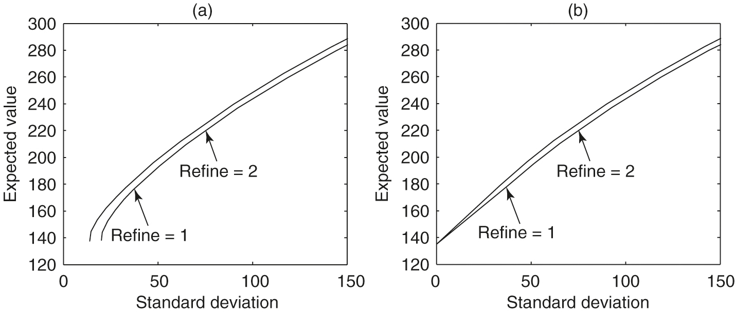
5.1 Effects of the improved interpolation scheme for the PDE method

In this subsection, we discuss the effects on numerical results of the linear interpolation scheme described in Section 4.4. We plot expected values against standard deviation, since both variables have the same units. Figure 1(a) illustrates the numerical efficient frontiers obtained using standard linear interpolation. It is clear that the results are very inaccurate for small standard deviations. It appears that the numerical methods were not able to construct the known point on the exact efficient frontier

$$({\mathrm{Var}}_{p^{*}(\cdot )}^{x,t}[W(T)],E_{p^{*}(\cdot )}^{x,t}[W(T)])=(0,w_0{\mathrm{e}}^{rT})\approx (0,134.9859).$$

This trivial case corresponds to the case where $\gamma ={\gamma }_{\min }$ (4.1), and the investor invests only in the risk-free bond and not in the risky asset. However, as shown in Figure 1(a), in this special case, the standard deviation obtained by the numerical scheme using standard linear interpolation is far from the exact solution.

Figure 1(b) shows the numerical efficient frontiers obtained with the improved linear interpolation scheme, where Algorithm 1 is utilized. It is obvious that the numerical efficient frontiers obtained with the improved linear interpolation scheme are more reasonable, especially for the small standard deviation region. In particular, the special point at which the variance is zero is now approximated accurately. This result illustrates the importance of using the optimal embedded terminal wealth $W_{\text{opt}}(t)$ and its function value for linear interpolation in constructing accurate numerical efficient frontiers. In all our numerical experiments in the following, the improved linear interpolation scheme is used.

Figure 1: Close-up of efficient frontier for small standard deviations. (a) No special interpolation. (b) Special interpolation.

5.2 Convergence analysis

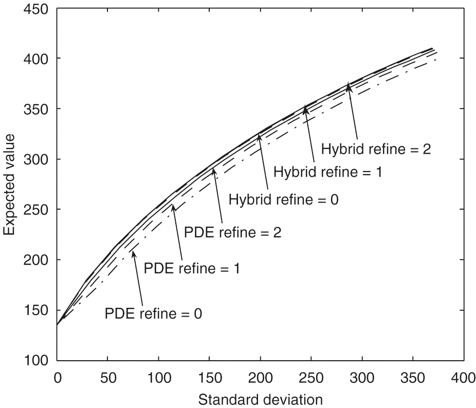
In this section, we illustrate the convergence of our numerical scheme and compare the performance of two methods, namely the PDE method (Section 4.2.1) and the hybrid method (4.2.2), for constructing the mean–variance frontier under our model setup.

Figure 2 shows that the mean standard deviation efficient frontiers computed by both the PDE method and the hybrid method converge to the same frontier as the computational grid is refined. Our numerical results demonstrate that the hybrid frontiers in general converge faster to the limit results than the pure PDE solutions. This same phenomenon was observed in Tse et al (2013). As shown in Figure 2, the frontiers obtained by the hybrid method are almost identical for refinement levels 1 and 2. Note that for both methods the optimal control is always computed by solving the HJB PDEs.

Table 5: The convergence table for the PDE method. [Small standard deviation (SD) case with $\gamma =\text{540}$.]

Refine	Mean	Change	Ratio	SD	Change	Ratio
0	207.1434			71.3924
1	210.4694	3.3260		65.5090	$-$5.88336
2	212.1957	1.7263	1.92	62.0862	$-$3.42288	1.72
3	213.1481	0.95238	1.81	60.4738	$-$1.61237	2.12

Table 6: The convergence table for the hybrid method. [Small standard deviation (SD) case with $\gamma =\text{540}$.]

Refine	Mean	Change	Ratio	SD	Change	Ratio
0	212.2993			56.6128
1	213.2077	0.908		57.7652	1.152
2	213.7573	0.550	1.65	58.2987	0.534	2.16
3	213.9903	0.233	2.36	58.5253	0.227	2.35

Table 7: The convergence table for the PDE method. [Large standard deviation (SD) case with $\gamma =\text{1350}$.]

Refine	Mean	Change	Ratio	SD	Change	Ratio
0	320.5139			217.0009
1	325.5443	5.030		212.1886	$-$4.812
2	328.2670	2.723	1.85	209.8434	$-$2.345	2.05
3	329.8172	1.550	1.76	208.9045	$-$0.939	2.50

Figure 2: Convergence of frontiers in the PDE method and the hybrid method. The frontiers labeled with “PDE” are obtained from the PDE method (Section 4.2.1). The frontiers labeled with “Hybrid” (Section 4.2.2) are obtained from a Monte Carlo simulation that uses the optimal controls determined by solving the HJB equation (2.15).

The same time steps are used in both the PDE method and Monte Carlo simulations for each refinement level. For example, the frontiers labeled with “$\text{Refine}=1$” for both methods in Figure 2 use the time steps specified as “Refinement 1” in Table 4. To achieve small sampling error in Monte Carlo simulations, ${10}^6$ simulations are performed for the numerical experiments. The standard error in Figure 2 can then be estimated. For example, consider a point on the frontier with a large standard deviation value that is about $350$. For the expected value of $W(T)$, the sample error is approximately $350/\sqrt{{10}^6}\approx 0.35$, which could be negligible in Figure 2.

We will verify our conclusion by examining several specific points on these efficient frontiers in Figure 2. Tables 5 and 6 show computed means and standard deviations for different refinement levels when $\gamma =540$. The numerical results indicate first-order convergence is achieved for both the PDE method and the hybrid method. In this case, our numerical results demonstrate that the hybrid frontiers converge faster to the limit results than the PDE solutions. Tables 7 and 8 show computed means and standard deviations for different refinement levels when $\gamma =1350$. The numerical results indicate first-order convergence is achieved for the PDE method. In this case, our numerical results also demonstrate that the hybrid frontiers converge faster to the limit results than the PDE solutions. However, the convergence ratio for the hybrid method is erratic. As we noted before, in this case, the sample error for the estimate of the mean value is about $0.2\simeq 200/\sqrt{{10}^6}$, which makes the convergence ratio estimates in Table 8 unreliable. To decrease the sample error to, for example, $0.02$, the number of simulation paths would have to increase to $100\times {10}^6$, which is unaffordable in terms of the computational cost. Note that in the case $\gamma =540$, with the small standard deviation, the sample error for the mean is about $0.05\simeq 50/\sqrt{{10}^6}$.

Table 8: The convergence table for the hybrid method. [Large standard deviation (SD) case with $\gamma =\text{1350}$.]

Refine	Mean	Change	Ratio	SD	Change	Ratio
0	329.4411			206.0875
1	330.5172	1.076		206.8351	0.748
2	330.7066	0.189	5.68	207.1958	0.361	2.07
3	331.2820	0.575	0.33	207.3707	0.175	2.06

Figure 3: Sensitivity analysis of the efficient frontiers with respect to different leverage constraints $p_{\text{max}}$. The Heston parameters and remaining model parameters are given in Tables 2 and 3. The hybrid method with discretization level 2 is used.

Remark 5.1 (Efficiency of the hybrid method).

We remind the reader that for both the hybrid and PDE methods, the same (computed) control is used. The more rapid convergence of the hybrid method is simply due to a more accurate estimate of the expected quantities (with a known control). This result is somewhat counterintuitive, since it suggests that a low accuracy control can be used to generate high accuracy expected values. We also observe this from the fact that a fairly coarse discretization of the admissible set ${?}_h$ generates fairly accurate solutions.

5.3 Sensitivity of efficient frontiers

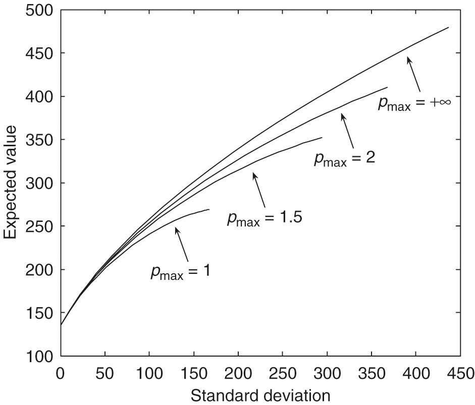
In this subsection, we show some numerical sensitivity analysis for the major market parameters, namely the leverage constraints $p_{\max }$, the market risk $\xi$, the mean reversion level for the variance $\theta$, the volatility of the variance $\sigma$, the correlation $\rho$ between the risky asset and the variance, and the mean reversion speed $\kappa$. In our numerical tests, the corresponding frontiers are generated as the market parameter of interest changes, and the values of the remaining parameters are fixed and listed in Tables 2 and 3. We use the hybrid method with discretization level 2.

Figure 4: Sensitivity analysis of the efficient frontiers with respect to different risk premium factor $\xi$ values. The remaining Heston parameters and model parameters are given in Tables 2 and 3. The hybrid method with discretization level 2 is used.

Figure 5: Sensitivity analysis of the efficient frontiers with respect to different mean reversion level $\theta$ values. The remaining Heston parameters and model parameters are given in Tables 2 and 3. The hybrid method with discretization level 2 is used.

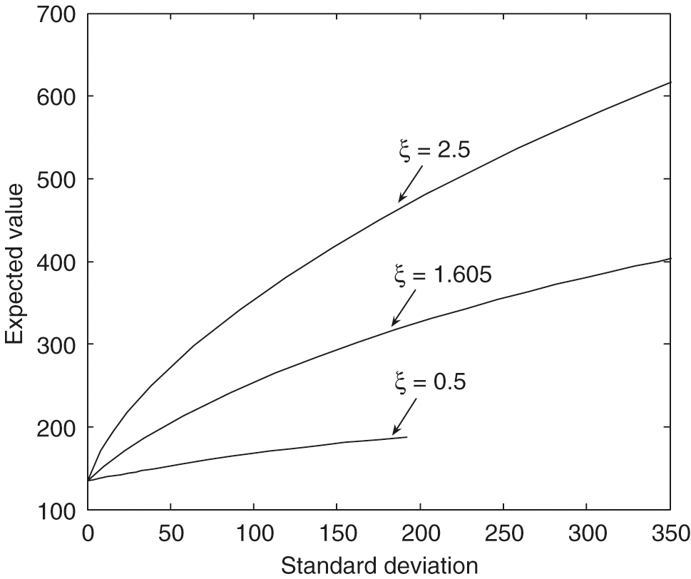
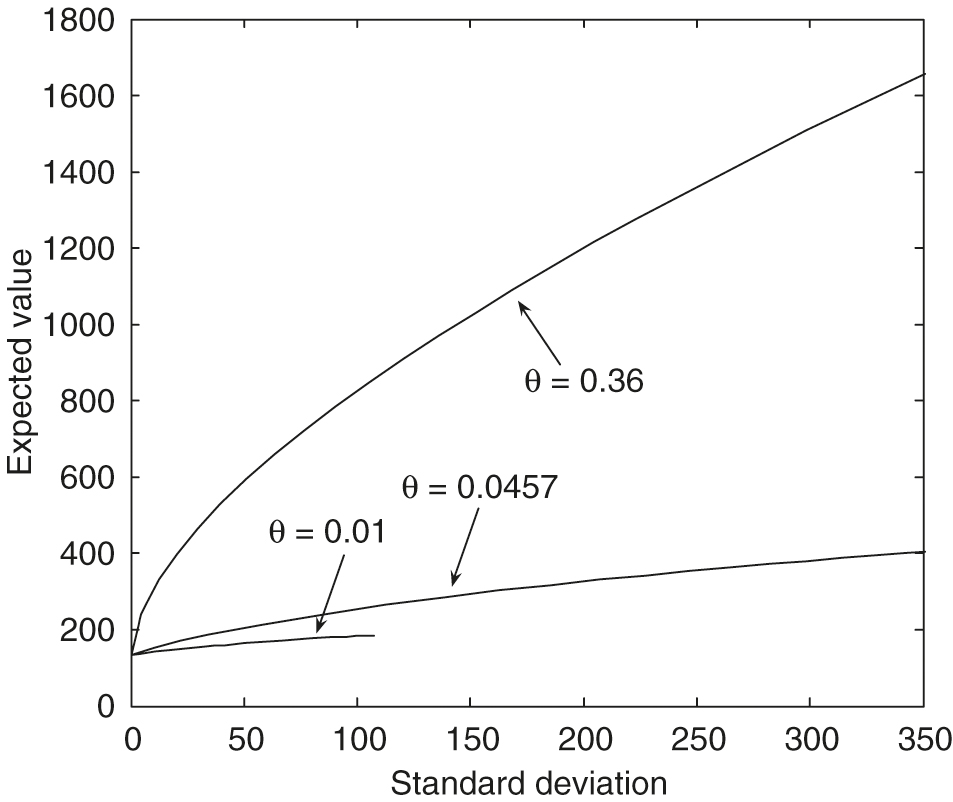
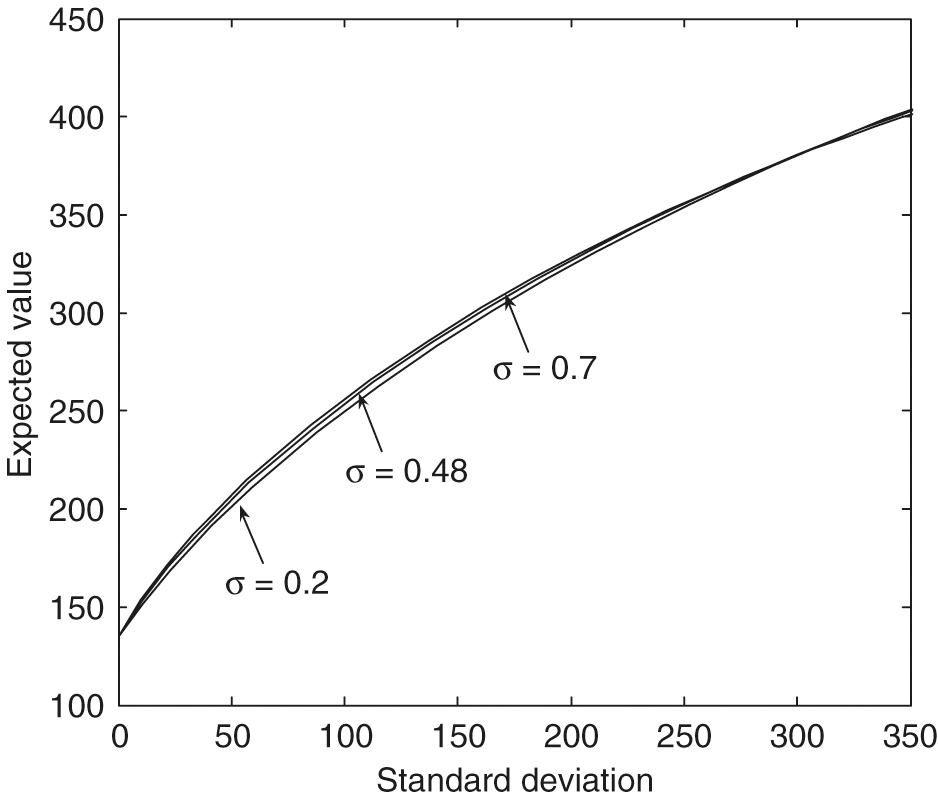
As observed in Figure 3, with $p_{\max }=\{1,1.5,2,+\mathrm{\infty }\}$, we can see that larger values of the leverage constraints $p_{\max }$ result in much more dominant efficient frontiers. From Figure 4, with $\xi =\{0.5,1.605,2.5\}$, we can see that larger values of $\xi$ result in much more dominant efficient frontiers. The maximal standard deviation point ($\gamma =+\mathrm{\infty }$) on the efficient frontier with $\xi =0.5$ is only about $191$, which is much smaller than those with larger $\xi$ values. From Figure 5, $\theta =\{0.01,0.0457,0.36\}$, we can see that larger values of the mean reversion level $\theta$ for the variance result in much more dominant efficient frontiers. The maximal standard deviation point ($\gamma =+\mathrm{\infty }$) on the efficient frontier with $\theta =0.01$ is only about $108$, which is much smaller than those with larger $\theta$ values. From Figure 6, $\sigma =\{0.2,0.48,0.7\}$, we can see that larger values of the volatility of the variance $\sigma$ result in slightly more dominant, efficient frontiers in general. In particular, these efficient frontiers in the large standard deviation region with different $\sigma$ values are almost identical.

Figure 6: Sensitivity analysis of the efficient frontiers with respect to different $\sigma$ values. The remaining Heston parameters and model parameters are given in Tables 2 and 3. The hybrid method with discretization level 2 is used.

Figure 7: Sensitivity analysis of the efficient frontiers with respect to different $\rho$ values. The remaining Heston parameters and model parameters are given in Tables 2 and 3. The hybrid method with discretization level 2 is used.

Figure 8: Sensitivity analysis of the efficient frontiers with respect to different $\kappa$ values. The Heston parameters and remaining model parameters are given in Tables 2 and 3. The hybrid method with discretization level 2 is used.

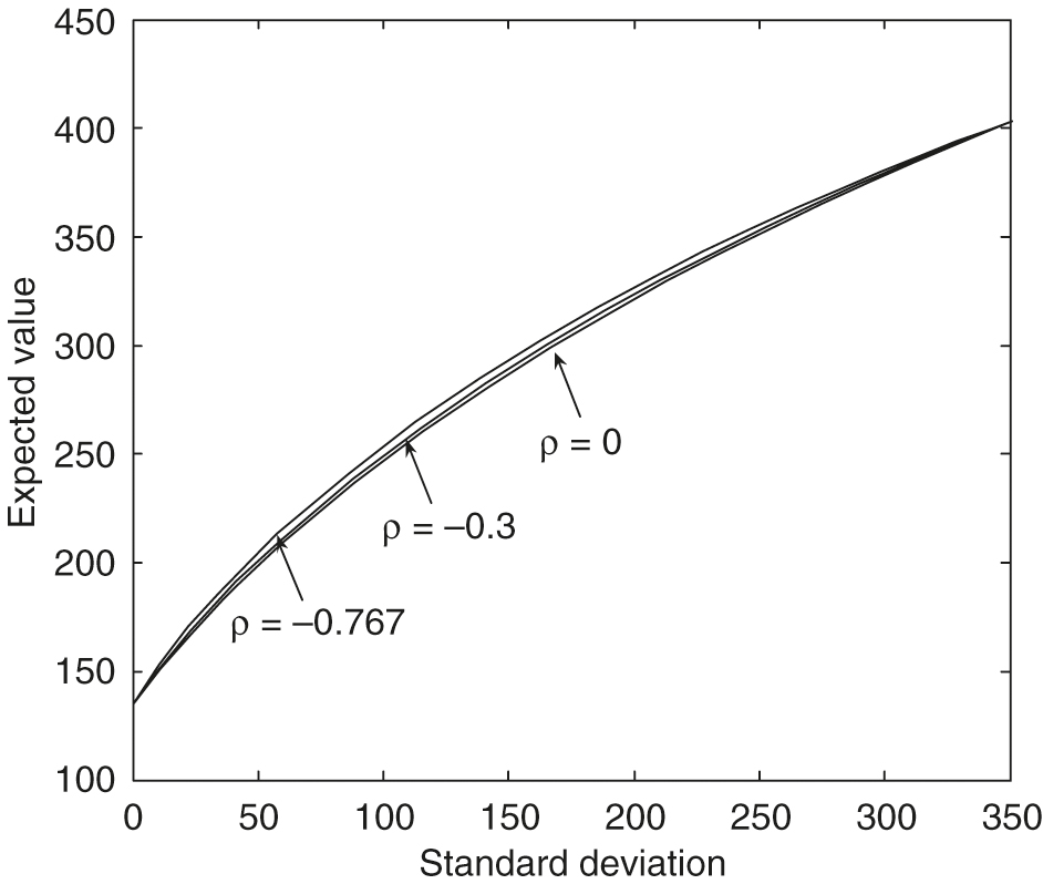
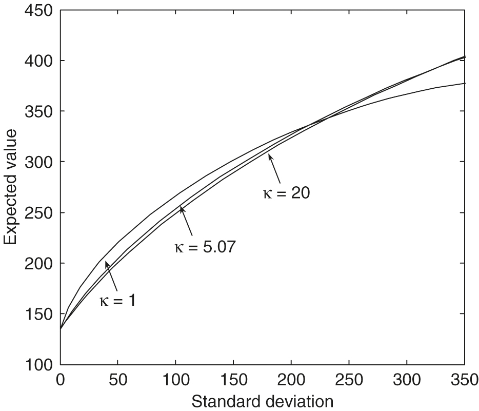
However, from Figure 7, with $\rho =\{-0.767,-0.3,0\}$, we can see that an increase in the correlation $\rho$ produces frontiers with a slightly smaller expected value for a given standard deviation. These efficient frontiers in the large standard deviation region with different $\rho$ values are almost identical. The effect of the $\kappa$ values on the efficient frontiers is more complex. From Figure 8, $\kappa =\{1,5.07,20\}$, in the small standard deviation region, an increase in $\kappa$ produces frontiers with a smaller expected value for a given standard deviation. However, when the standard deviation increases to about $230$, the larger values of $\kappa$ gradually result in more significant dominant efficient frontiers.

5.4 Comparison between constant volatility and stochastic volatility cases

In this paper, the risky asset follows the stochastic volatility model ((2.2) and (2.3)). In this section, we will compare the constant volatility and stochastic volatility cases in terms of mean–variance efficiency for the continuous-time pre-commitment mean–variance problem. With a constant volatility, the risky asset is governed by the following GBM process:

$$\frac{\mathrm{d}S}{S}=(r+\mu )\mathrm{d}t+{\sigma }_S\mathrm{d}{Z}_s.$$

(5.1)

To compare this with the stochastic volatility case in Table 2, the constant volatility ${\sigma }_S$ is set to $\sqrt{\theta }\approx 0.2138$, and the risky return over the risk-free rate $\mu$ is set to $\xi {\sigma }_S^2=0.0733485$, which has the same mean premium of the volatility risk as the stochastic volatility model (2.2). This then corresponds to the case where the variance $V(t)$ in (2.2) is fixed to the mean reversion level $\theta$. The remaining mean–variance problem parameters are the same as those listed in Table 3.

Figure 9: Efficient frontier comparison between constant volatility and stochastic volatility cases. For the stochastic volatility cases, $\kappa =\text{1},\text{5.07}$; the remaining stochastic volatility parameters are given in Table 2. The GBM parameters are given in Section 5.4.

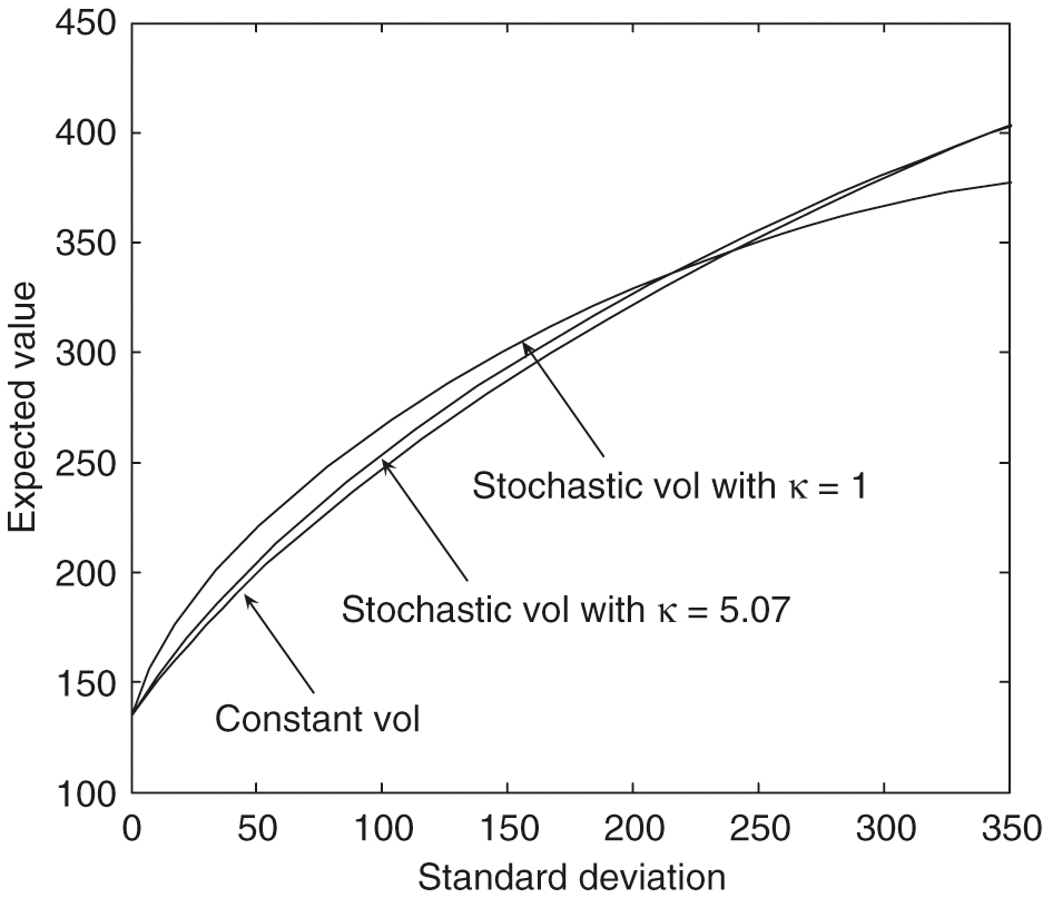
Figure 9 illustrates the fact that the efficient frontiers produced by using the stochastic volatility slightly dominate the curve produced by the constant volatility model. With the Heston model’s parameters in Table 2, we may conclude that the efficient frontier produced by the constant volatility is a good approximation of the frontier generated by the stochastic volatility model. From Figure 9, however, we see that if the mean reversion speed $\kappa$ is set to a small value, eg, 1, in the stochastic volatility case, the efficient frontiers computed using a constant volatility model will be considerably different from those computed using the stochastic volatility model. The quantity $1/\kappa$ is measured in years and is related to the time over which a volatility shock dissipates. Specifically, the half-life of a volatility shock is $(\ln 2)/\kappa$.

Finally, using the portfolio allocation strategy that is precomputed and stored from the constant volatility case, we then carry out a Monte Carlo simulation where the risky asset follows the stochastic volatility model. We then compare the results using this approximate control, with the optimal control computed using the full stochastic volatility model. From Table 9, we can see that the mean–variance pairs computed using the optimal strategy are very close to the strategy computed using the GBM approximation. Based on several tests, a good heuristic guideline is that if $\kappa T>40$, then the GBM control is a good approximation to the exact optimal control.

Table 9: Given a $\gamma$, the optimal portfolio allocation strategy is computed and stored assuming a control process, which is either GBM or stochastic volatility (SV). [The mean–variance pairs are estimated by Monte Carlo simulation, using the stored controls, assuming that the actual price process follows either GBM or stochastic volatility. For the stochastic volatility case, the parameters are given in Table 2. For the GBM case, the variance is fixed to the mean value of the stochastic volatility case. SD denotes standard deviation.]

		$?\mathbf{=}\text{???}$		$?\mathbf{=}\text{????}$
Control process	Price process	Mean	SD	Mean	SD
GBM	GBM	209.50	59.68	330.09	213.01
GBM	SV	212.68	58.42	329.13	207.23
SV	SV	213.99	58.53	331.28	207.37

6 Conclusion

In this paper, we develop an efficient fully numerical PDE approach for the pre-commitment continuous-time mean–variance asset allocation problem when the risky asset follows a stochastic volatility model. We use the wide stencil method (Ma and Forsyth 2014) to overcome the main difficulty in designing a monotone approximation. We show that our numerical scheme is monotone, consistent and ${\mathrm{\ell }}_{\mathrm{\infty }}$-stable. Hence, the numerical solution is guaranteed to converge to the unique viscosity solution of the corresponding HJB PDE, assuming that the HJB PDE satisfies a strong comparison property. Further, using semi-Lagrangian time stepping to handle the drift term, along with an improved method of linear interpolation, allows us to compute accurate efficient frontiers. When tracing out the efficient frontier solution of our problem, we demonstrate that the hybrid (PDE–Monte Carlo) method (Tse et al 2013) converges faster than the pure PDE method. Similar results are observed in Tse et al (2013). Finally, if the mean reversion time $1/\kappa$ is small compared with the investment horizon $T$, then a constant volatility GBM approximation to the stochastic volatility process gives a very good approximation to the optimal strategy.

Declaration of interest

The authors report no conflicts of interest. The authors alone are responsible for the content and writing of the paper. This work was supported by the Bank of Nova Scotia and the Natural Sciences and Engineering Research Council of Canada.

References

• Aït-Sahalia, Y., and Kimmel, R. (2007). Maximum likelihood estimation of stochastic volatility models. Journal of Financial Economics 83(2), 413–452 (http://doi.org/b3c4dg).
• Barles, G., and Souganidis, P. E. (1991). Convergence of approximation schemes for fully nonlinear second order equations. Asymptotic Analysis 4(3), 271–283.
• Basak, S., and Chabakauri, G. (2010). Dynamic mean–variance asset allocation. Review of Financial Studies 23(8), 2970–3016 (http://doi.org/cqnc3g).
• Bauerle, N., and Grether, S. (2015). Complete markets do not allow free cash flow streams. Mathematical Methods of Operations Research 81, 137–145 (http://doi.org/bkpx).
• Bielecki, T. R., Jin, H., Pliska, S. R., and Zhou, X. Y. (2005). Continuous-time mean–variance portfolio selection with bankruptcy prohibition. Mathematical Finance 15(2), 213–244 (http://doi.org/cj3svf).
• Bjork, T., and Murgoci, A. (2010). A general theory of Markovian time inconsistent stochastic control problems. SSRN Working Paper (http://doi.org/fzcfp2).
• Breeden, D. T. (1979). An intertemporal asset pricing model with stochastic consumption and investment opportunities. Journal of Financial Economics 7(3), 265–296 (http://doi.org/c8t9tr).
• Chen, Z. L., and Forsyth, P. A. (2007). A semi-Lagrangian approach for natural gas storage valuation and optimal operation. SIAM Journal on Scientific Computing 30(1), 339–368 (http://doi.org/bqnf83).
• Cox, J. C., Ingersoll, J., Jonathan, E., and Ross, S. A. (1985). A theory of the term structure of interest rates. Econometrica: Journal of the Econometric Society 53(2), 385–407 (http://doi.org/cbb2pm).
• Cui, X., Li, D., Wang, S., and Zhu, S. (2012). Better than dynamic mean–variance: time inconsistency and free cash flow stream. Mathematical Finance 22(2), 346–378 (http://doi.org/dvr3gq).
• Dang, D. M., and Forsyth, P. A. (2014a). Better than pre-commitment mean–variance portfolio allocation strategies: a semi-self-financing Hamilton–Jacobi–Bellman equation approach. European Journal on Operational Research 132, 271–302 (http://doi.org/bkpk).
• Dang, D. M., and Forsyth, P. A. (2014b). Continuous time mean–variance optimal portfolio allocation under jump diffusion: a numerical impulse control approach. Numerical Methods for Partial Differential Equations 30(2), 664–698 (http://doi.org/bkpz).
• Dang, D. M., Forsyth, P. A., and Li, Y. (2016). Convergence of the embedded mean–variance optimal points with discrete sampling. Numerische Mathematik 132(2), 271–302 (http://doi.org/bkp2).
• Debrabant, K., and Jakobsen, E. (2013). Semi-Lagrangian schemes for linear and fully non-linear diffusion equations. Mathematics of Computation 82(283), 1433–1462 (http://doi.org/bkp3).
• d’Halluin, Y., Forsyth, P. A., and Labahn, G. (2004). A penalty method for American options with jump diffusion processes. Numerische Mathematik 97(2), 321–352 (http://doi.org/d5sn5v).
• Douglas, J. J., and Russell, T. F. (1982). Numerical methods for convection-dominated diffusion problems based on combining the method of characteristics with finite element or finite difference procedures. SIAM Journal on Numerical Analysis 19(5), 871–885 (http://doi.org/dzghv5).
• Ekström, E., and Tysk, J. (2010). The Black–Scholes equation in stochastic volatility models. Journal of Mathematical Analysis and Applications 368(2), 498–507 (http://doi.org/drbjzd).
• Feller, W. (1951). Two singular diffusion problems. Annals of Mathematics 54(1), 173–182 (http://doi.org/bvf5m4).
• Forsyth, P. A., and Labahn, G. (2007). Numerical methods for controlled Hamilton–Jacobi–Bellman PDEs in finance. The Journal of Computational Finance 11(2), 1–44 (http://doi.org/bkp4).
• Heston, S. L. (1993). A closed-form solution for options with stochastic volatility with applications to bond and currency options. Review of Financial Studies 6(2), 327–343 (http://doi.org/fg525s).
• Huang, Y., Forsyth, P. A., and Labahn, G. (2012). Combined fixed point and policy iteration for HJB equations in finance. SIAM Journal on Numerical Analysis 50(4), 1849–1860 (http://doi.org/bkp5).
• Kahl, C., and Jäckel, P. (2006). Fast strong approximation Monte Carlo schemes for stochastic volatility models. Quantitative Finance 6(6), 513–536 (http://doi.org/cqtf4z).
• Li, D., and Ng, W.-L. (2000). Optimal dynamic portfolio selection: multiperiod mean–variance formulation. Mathematical Finance 10(3), 387–406 (http://doi.org/dt4h2f).
• Lord, R., Koekkoek, R., and Dijk, D. V. (2010). A comparison of biased simulation schemes for stochastic volatility models. Quantitative Finance 10(2), 177–194 (http://doi.org/bjjn3n).
• Ma, K., and Forsyth, P. A. (2014). An unconditionally monotone numerical scheme for the two factor uncertain volatility model. IMA Journal on Numerical Analysis (forthcoming).
• Nguyen, P., and Portait, R. (2002). Dynamic asset allocation with mean variance preferences and a solvency constraint. Journal of Economic Dynamics and Control 26(1), 11–32 (http://doi.org/dgkfgc).
• Pironneau, O. (1982). On the transport-diffusion algorithm and its applications to the Navier-Stokes equations. Numerische Mathematik 38(3), 309–332 (http://doi.org/dz4dc9).
• Pooley, D. M., Forsyth, P. A., and Vetzal, K. R. (2003). Numerical convergence properties of option pricing PDEs with uncertain volatility. IMA Journal of Numerical Analysis 23(2), 241–267 (http://doi.org/bq6t6z).
• Saad, Y. (2003). Iterative Methods for Sparse Linear Systems. SIAM (http://doi.org/bq25g6).
• Tse, S. T., Forsyth, P. A., Kennedy, J. S., and Windcliff, H. (2013). Comparison between the mean–variance optimal and the mean-quadratic-variation optimal trading strategies. Applied Mathematical Finance 20(5), 415–449 (http://doi.org/bkp6).
• Tse, S. T., Forsyth, P. A., and Li, Y. (2014). Preservation of scalarization optimal points in the embedding technique for continuous time mean variance optimization. SIAM Journal on Control and Optimization 52(3), 1527–1546 (http://doi.org/bkp7).
• Varga, R. S. (2009). Matrix Iterative Analysis, Volume 27. Springer.
• Vigna, E. (2014). On efficiency of mean–variance based portfolio selection in defined contribution pension schemes. Quantitative Finance 14(2), 237–258 (http://doi.org/bkp8).
• Wang, J., and Forsyth, P. A. (2008). Maximal use of central differencing for Hamilton–Jacobi–Bellman PDEs in finance. SIAM Journal on Numerical Analysis 46(3), 1580–1601 (http://doi.org/ffw87k).
• Wang, J., and Forsyth, P. A. (2010). Numerical solution of the Hamilton–Jacobi–Bellman formulation for continuous time mean variance asset allocation. Journal of Economic Dynamics and Control 34(2), 207–230 (http://doi.org/d2s8c8).
• Wang, J., and Forsyth, P. A. (2012). Comparison of mean variance like strategies for optimal asset allocation problems. International Journal of Theoretical and Applied Finance 15(2), 1250014 (http://doi.org/bhwk).
• Zhao, Y., and Ziemba, W. T. (2000). Mean–variance versus expected utility in dynamic investment analysis. Working Paper, University of British Columbia.
• Zhou, X. Y., and Li, D. (2000). Continuous-time mean–variance portfolio selection: a stochastic LQ framework. Applied Mathematics and Optimization 42(1), 19–33 (http://doi.org/b6r9zv).

Download PDF

• Keywords
• Computational finance
• Mean variance
• Stochastic volatility
• Original research