Forward volatility: a model-free framework for hedging options risk

TS Imagine – Volatility Research describes a model-free framework that extracts forward volatility directly from option prices, providing a zero-cost static hedge that isolates and manages future volatility risk across maturities

Introduction

Risk managers use forwards to organise risk. An equity or foreign exchange forward is a price fixed today for delivery later, replicated by a static position in spot and cash. No dynamics assumption is required: no-arbitrage alone pins the price down, and every desk agrees on it.

Options carry no such anchor: any answer to ‘what will my book look like in three months?’ requires a model of the dynamics, and desks disagree. This feature constructs the missing reference – a forward volatility curve extracted from current option prices with no modelling assumption – and shows it is achievable by an explicit, zero-cost static hedge.

Implied probability density functions

We work throughout in log-moneyness k = ln(K/F), with the forward at k = 0; this centres the smile at the origin and simplifies every formula that follows. A call is then:

where c(k) is the price per unit of forward. The discount factor and the forward enter every expression below as the same two multipliers, so we suppress them and work with c(k) throughout.

An option’s smile and its implied risk-neutral density p(k) carry the same information¹, p(k) is the second strike-derivative of the call price. The density is the more useful of the two: it is the price, per unit notional, of an infinitesimal butterfly struck at k – a payoff converging to a Dirac delta at expiry. We write [p(k)dk] for an actual butterfly, of value p(k)dk – used throughout. Any payoff f(k) is therefore priced and hedged as ∫f(k)·[p(k)dk].

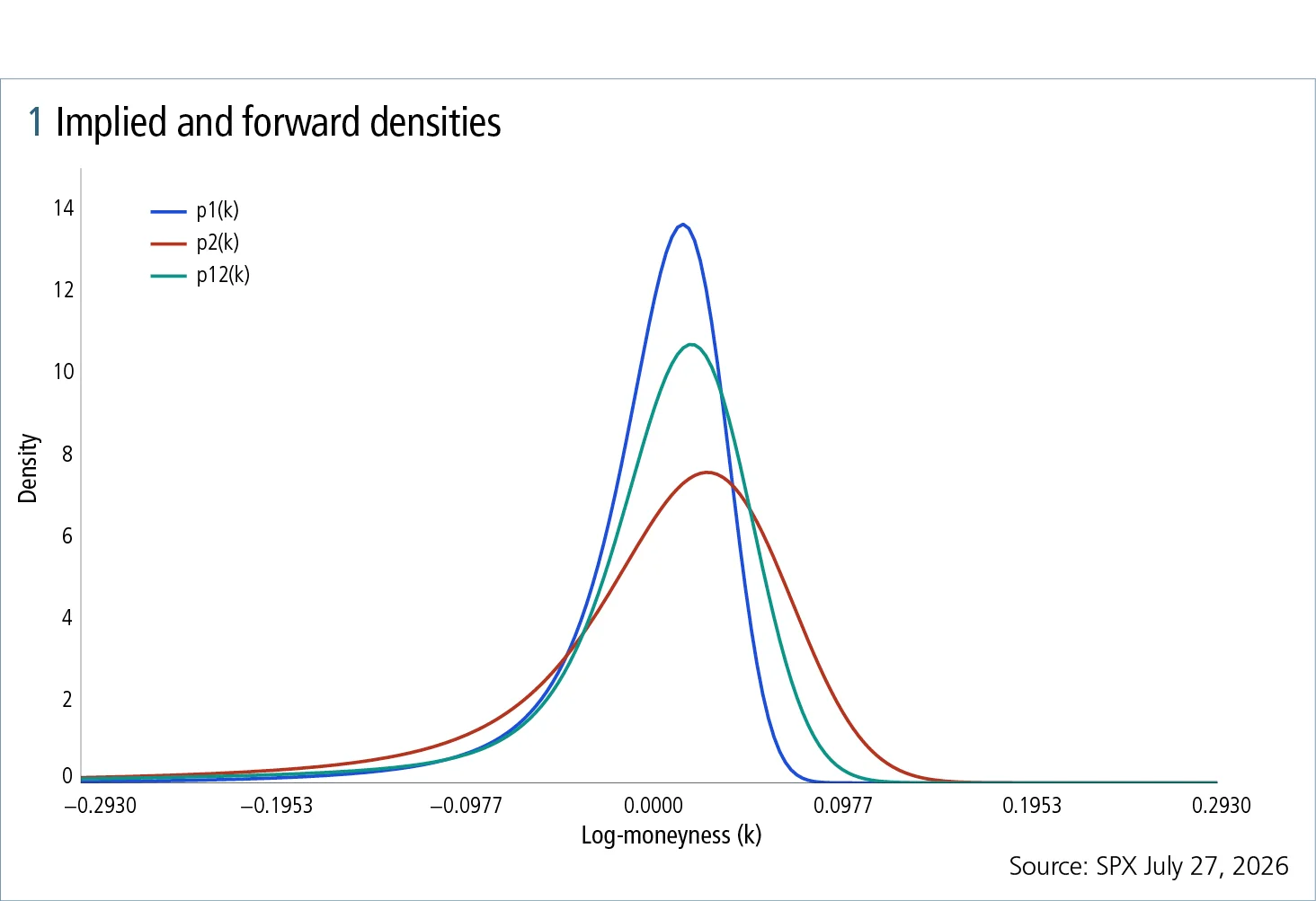
The forward density p_₁₂(k) – prevailing over [T_₁,T_₂] – is pinned down by the convolution: the T_₂ outcome is the T_₁ outcome convolved with the move over the forward period.

Solved by Fourier transform, φ₁₂ = φ₂/φ₁, then inverse transform, with light smoothing to remove deconvolution artefacts. Reconvolving p_₁₂ with p_₁ reproduces p_₂ to within 0.1% of its mass on real S&P 500 (SPX) data. Figure 1 plots all three:

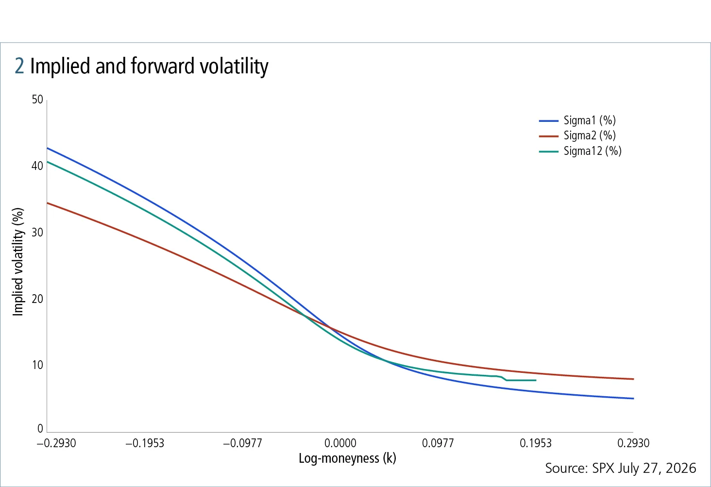
Implied vol follows in two steps: integrating each density against the call payoff gives c_₁(k), c_₂(k), and c_₁₂(k); inverting each through Black-Scholes gives σ_₁, σ_₂, and σ_₁₂, the forward volatility curve over [T_₁,T_₂]. Figure 2 plots all three.

Fundamental equation

The same construction, on call prices rather than densities, delivers the paper’s central result.

Write the T_₂ call as an integral over forward-weighted T_₁ butterflies, each weighted by the forward call price c_₁₂:

The eᵏ′ is a unit conversion: the butterfly [eᵏ′p_₁(k′)dk′] pays the realised T_₁ level, the unit c_₁₂ is quoted in. Its weights integrate to one – with p = d²C/dK², ∫eᵏp(k)dk integrates by parts to the zero-strike call, which must equal the forward. p_₁ and p_₂ inherit that from the listed calls behind them; the convolution passes it to p_₁₂.

Mark each side as a traded position – in brackets – and take the difference, that is the fundamental equation, zero for every strike today, now written as an options position:

The right is a strip of forward-weighted T_₁ butterflies [eᵏ′p_₁(k′) dk′], each held in the quantity c_₁₂(k−k′) – a price, not a traded quantity. Both terms have identical value today, so the position – long the T_₂ call, short the strip, the forward-vol contract – costs nothing at inception.

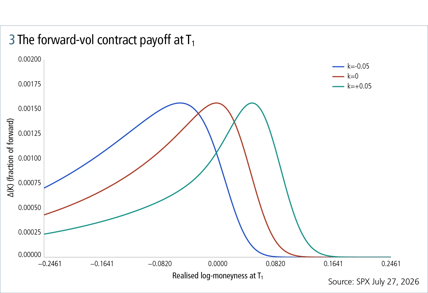
Project forward to T_₁, over a range of realised stock prices. At the forward, the difference is no longer zero: it is the gap between the forward call price under the vol curve that actually realises and the curve locked in today:

This is a clean, one-dimensional bet on the level of the forward vol curve. Figure 3 plots Δ(k) at T_₁ for the T_₁ = 25, T_₂ = 81-day pair (SPX July 27, 2026), under an illustrative +1.0 vol-point shock.

Because each contract is individually zero-cost, any linear combination across strikes is zero-cost too – a trader can assemble, at no premium, an arbitrary target vega profile by choosing quantities at a handful of strikes.

Hedging an options portfolio

This is where the framework becomes operational. The unrealised profit and loss (P&L) of an options portfolio P over [0,T_₁] decomposes as:

where Σ_f is the forward surface locked in today and Σ₁ is whatever prevails at T_₁. The first bracket is the P&L if volatility evolved onto the model-free forward – realised-spot risk only. The second is pure volatility risk: the realised surface’s deviation from the locked-in forward, conditional on spot. The fundamental equation replicates the first term at zero cost, supplying an overlay that isolates – and can neutralise – the second.

A single ‘portfolio vega’ is misleading: a three-month and a three-year option both carry vega, but summing them is a category error, like netting the dollar value of a basis point across maturities. Figure 4 takes a realistic multi-expiry SPX book – 72 option legs and four forward hedges, September to December 2026 – and decomposes its forward vega by expiry and in aggregate: each maturity contributes a differently shaped curve in spot and vega.

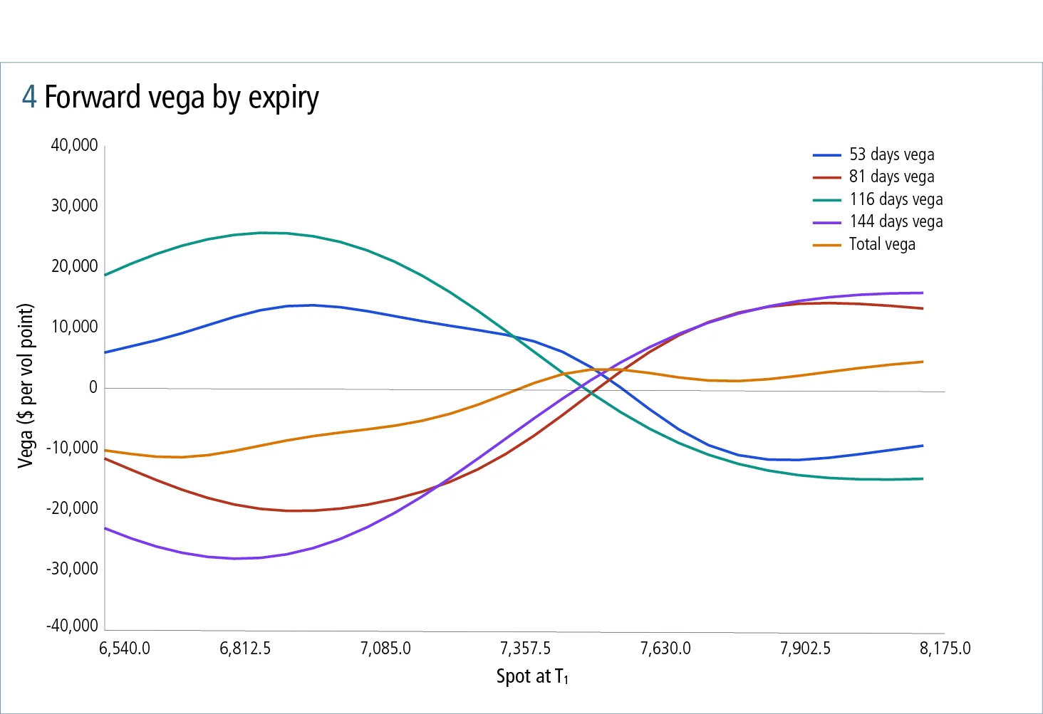
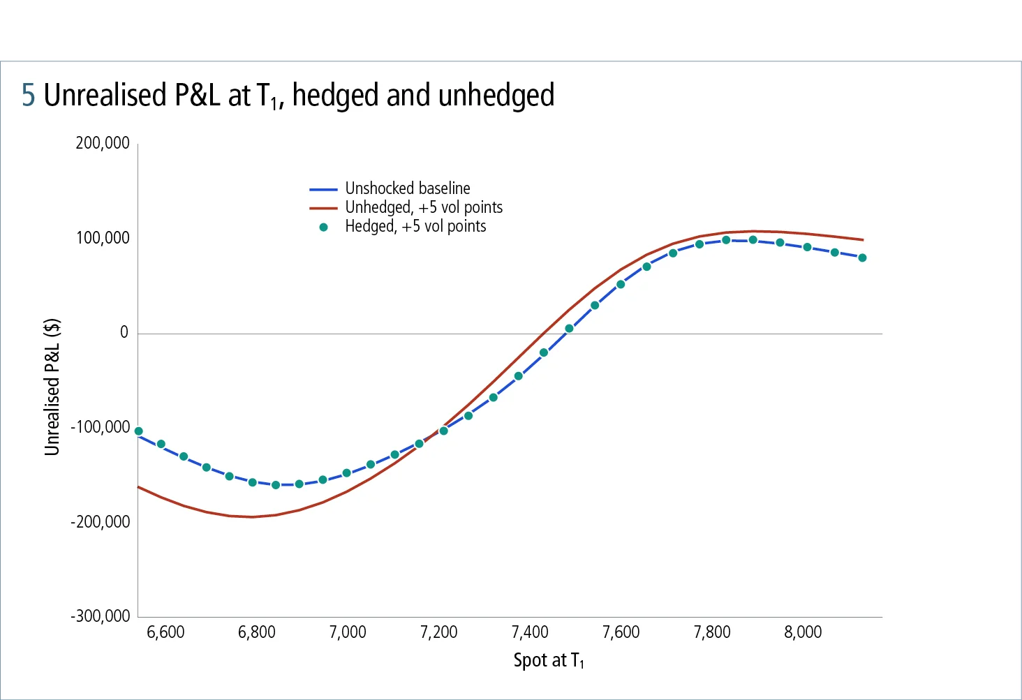
The fundamental equation modifies this profile at zero cost; here we zero out vega. Figure 5 fits an independent seven-contract strip to that target at each expiry and tests the combined hedge under a +5 vol-point shock: the hedged curve stays close to the unshocked baseline while the unhedged book drifts on the downside.

Forward-starting options: completing the circle

A forward-starting option – struck at eᵏ·F_₁ when spot first arrives at T_₁, expiring at T_₂ – is worth exactly c_₁₂(k)·F_₁, the forward call price this article has built throughout. One could posit that a c_₂(k) call is the expected value of a strip of forward-starting calls, which would look exactly like the fundamental equation. But that is pedagogical, not a proof.

The actual proof is by dynamic hedging – and, notably, in options alone, with no position in the underlying stock. That omission matters: the result assumes nothing about how the stock moves. We know of no other dynamic-hedging argument that trades only options.

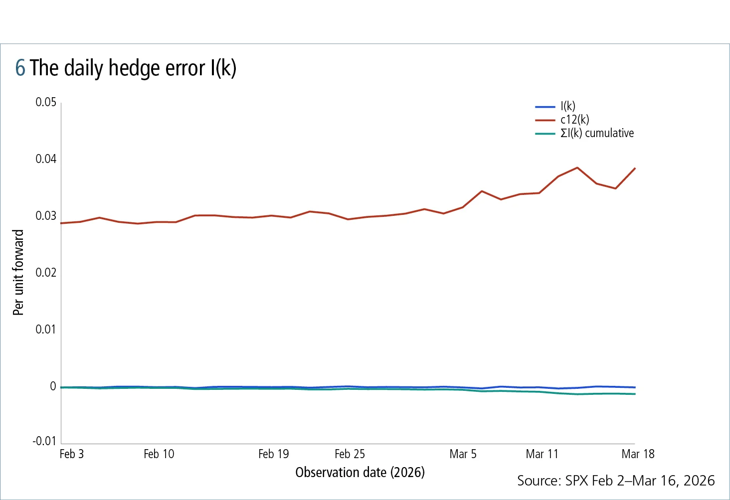
The result is established using the hedging portfolio [c_₁₂(k)·F_₁] − Δ(k): long the forward-starting option, short the zero-cost contract Δ(k) built above. Examining its value one period later – not just at expiry – shows this to be a self-financing hedging strategy with negligible error I(k).

We omit the error bound.² Figure 6 shows I(k) versus the forward-starting option price, measured daily over the T_₁ horizon, earlier in the same SPX sample.

<sup>1. DT Breeden and Litzenberger, RH (1978), Prices of state-contingent claims implicit in option prices, The Journal of Business, 51 (4), pp. 621–651.
2. Forward volatility III: Forward-starting options, TS Imagine – Volatility Research, working paper.</sup>