Journal of Investment Strategies
ISSN:
2047-1246 (online)
Editor-in-chief: Ali Hirsa
Need to know
- This paper focusses on how to construct optimal multi-factor equity portfolios.
- Portfolio optimization is used to enforce the targeted factor exposures and manage constraints.
- We demonstrate that only our proposed methodology can avoid betting on unintended factors.
- We show how to implement the approach with an illustration using portfolios exposed to four factors.
Abstract
This paper is devoted to the question of optimal portfolio construction for equity factor investing. The first part focuses on how to make sure that a given equity portfolio has the targeted factor exposures, even before imposing any constraints. We show that such portfolios can be derived from mean–variance optimization using expected stock returns as inputs, provided these are built in a robust way from information about the factors. We propose a framework to build those robust expected stock returns and show that the targeted factor exposures are retained by the portfolios both before and after applying realistic constraints, eg, long only. Other, more simplistic, approaches fail. The second part illustrates the application of the framework to a practical case, where the objectives are, first, to decide on the risk-budget allocation to factors in some pragmatic way and, second, to construct a long-only constrained portfolio that retains the targeted exposures to four factors from well-known asset-pricing equity models, namely high-minus-low (HML), robust-minus-weak (RMW), conservative-minus-aggressive (CMA) and momentum (MOM).
Introduction
1 Introduction
Factors are characteristics that explain the risk of stock and equity portfolio returns. According to financial theory from the 1950s that is consistent with the efficient market hypothesis, one factor – the market factor – should be all that is needed. However, empirical evidence that the exposure to the market factor as measured by beta is not sufficient has been available since Haugen and Heines (1972) showed that US stocks sharing the common characteristic of exhibiting the lowest volatility delivered higher returns than expected from their level of beta. Basu (1977) showed that value stocks, those exhibiting the lowest price-to-earnings ratio, also delivered higher returns than expected from their level of beta. Jagadeesh and Titman (1993) showed that momentum stocks, those with stronger past performances at horizons of twelve months, also delivered average returns higher than predicted by their beta. More recently, Novy-Marx (2013) established that stocks that share the characteristic of being the most profitable, ie, those with the highest gross profit, also delivered abnormally high returns despite their beta.
Hou et al (2017) listed 447 factors reported in the financial literature that are believed to have explanatory powers in the cross-section of stock returns. However, many of these factors overlap in terms of information content as they are just different ways of looking at the same characteristic. For that reason, they can be grouped into just a handful of independent styles such as value, quality, momentum or low risk. Others are either too difficult to replicate or not statistically significant, as pointed out by Hou et al (2017), or the result of data snooping, as highlighted by Harvey et al (2016).
Indeed, at the other end of the spectrum, Fama and French (2015) proposed that a parsimonious asset-pricing model for equities does not need more than five factors, while Blitz et al (2018) proposed a number of factors that was not much larger.
Evidence that myriad factors generate premiums uncorrelated with the equity market factor abounds in the academic literature, even if there is no consensus when it comes to explaining the source of those premiums. Some explain them as compensation from exposures to risks, others as resulting from behavioral preferences that create imbalances in the demand and offer of stocks sharing the common characteristics captured by a given factor.
Irrespective of the source of factor premiums, strategies that promise to outperform market capitalization indexes via shifts in favor of stocks exposed to factors such as those typically grouped into value, quality, momentum and low-risk styles have been growing in popularity. The so-called smart beta strategies get there indirectly by starting with algorithms for portfolio construction that land in portfolios with exposures to factors that pay premiums. As shown by Leote de Carvalho et al (2012), the risk and returns to minimum variance and maximum diversification portfolios can be explained by tilts toward low-risk stocks, whereas the risk and returns to risk parity portfolios can be explained by tilts toward smaller capitalization, low-risk and, to some extent, value stocks. In turn, factor investing focuses on building portfolios with targeted factor exposures. The line dividing smart beta and factor investing is tenuous, but the portfolio construction algorithms and the factor exposures, acquired passively in smart beta and actively targeted in factor investing, tend to make the difference.
Different approaches to building portfolios with multiple factor exposures have been put forward. Haugen and Baker (1996) proposed the use of cross-sectional regressions, which relies on past cross-sectional correlations of stock returns with stock exposures to factors in order to determine which factors are relevant and which are superfluous. In this framework, the last one-period cross-sectional stock returns are regressed against stock factor exposures at the start of that period. The approach is repeated at each rebalancing, typically monthly or quarterly. The regression produces the optimal factor weights that should be used to generate forecasts of stock returns for the next period. The expected stock returns are often used in mean–variance optimization to build a multifactor portfolio. Unfortunately, as highlighted by Leote de Carvalho (2016), there are three problems. First, the framework is not workable when similar characteristics are used as factors (eg, including factors from the same style, such as price-to-earnings and price-to-book as value factors). The problem stems from their strong correlation in the cross-section. Practitioners tend to dampen the cross-sectional factor correlations, but this defeats the purpose. Second, the weight of factors is volatile from one rebalancing to another unless it is averaged over a number of past periods, thus obliging factor weights to rely on momentum. Third, the expected stock returns are not robust, and thus, when used in mean–variance optimization, they lead to corner solutions, a problem that is solved in an unsatisfactory way by imposing constraints on stock weights. In addition, the optimal mean–variance portfolio exhibits a number of unwanted exposures to other risks.
Many practitioners prefer simpler approaches, eg, multiscoring approaches, that just calculate an average multifactor score for each stock based on the stock exposure to the factors chosen a priori. Factors are selected based on the empirical evidence of the premium they have generated. The final portfolio is often just an equally weighted selection of stocks with the highest average multifactor scores, recalculated monthly or quarterly. However, portfolios tend to exhibit systematic risk exposures that are not desired or controlled, eg, overreliance on smaller capitalization stocks, or a beta different from 1 and variable over time. Leote de Carvalho et al (2017) and Amenc et al (2018) highlighted the importance of controlling for beta in multifactor portfolios. Moreover, with such a simplistic approach, it is not easy to manage portfolio constraints such as turnover or setting the beta to .
Finally, some prefer to consider the multifactor scores for each stock at each rebalancing as proxies of expected stock returns in mean–variance optimization. Unfortunately, as we shall see, this approach suffers from the same problems as using stock returns derived from multifactor cross-sectional regressions.
One approach that became popular with practitioners is based on the idea that factor premiums can be captured efficiently with long–short portfolios that may be combined into a zero-sum long–short portfolio extension, which, when sitting next to the benchmark index, generates a tracking error and excess returns over that benchmark. This approach went by the name “130/30” since often the active extension corresponded to a 30/30 long–short portfolio. As described by Lo and Patel (2008), such approaches capture well the excess returns from stocks with negative exposures to factors that can be difficult to underweight in long-only portfolios. However, interest in these approaches, despite their simplicity, from investors and practitioners has faded considerably since the global financial crisis. This is because of counterparty risk and the costs of implementing the extension portfolio using total return swaps.
Leote de Carvalho et al (2014) proposed that implied stock returns derived by reverse optimization from the extension of 130/30 portfolios can be used in mean–variance optimization in order to efficiently build constrained multifactor portfolios, eg, long only. They showed that (i) these implied stock returns are robust for mean–variance optimization and (ii) their approach in effect minimizes the impact of portfolio constraints while retaining as much as possible the systematic factor risk exposures in the 130/30 portfolio from which the implied stock returns were derived.
Here, we focus on the optimal construction of multifactor equity portfolios: in particular, the question of how to make sure portfolios retain the desired factor exposures before and after applying constraints. We split this problem in two, as proposed by Leote de Carvalho et al (2014). First, we look at how to construct an optimal unconstrained multifactor equity portfolio with targeted factor exposures. Second, we investigate how to retain those factor exposures even after applying constraints, eg, long only.
In Section 2, we consider three approaches for generating stock returns from factor returns. First, we consider a naive approach, the simplest we could conceive of, whereby expected stock returns are calculated as the sum product of stock weights in each long–short factor portfolio by each respective expected factor return. This is a proxy of the multiscoring approach. It runs into trouble because, if we turn the problem around and try to calculate the factor returns from the derived stock returns using a similar naive approach, we find a different result from the starting point, ie, the problem is not reversible. In the other two examples, we impose the constraint that reversibility between stock and factor returns must hold. Since there is no unique way of imposing reversibility, we consider two approaches: (i) the simplest approach we could conceive of; and (ii) the approach of Leote de Carvalho et al (2014), which, indeed, satisfies the reversibility condition.
In Section 2, we also discuss the properties of unconstrained optimal mean–variance portfolios for each of the three approaches. We show that only the portfolios based on the approach of Leote de Carvalho et al (2014) have no exposure to factors other than those targeted. In the other two cases, the portfolios exhibit large exposure to factors orthogonal to those used to build the expected stock returns.
In Section 3, we show how to implement the approach of Leote de Carvalho et al (2014). We discard the other two approaches in view of their lack of robustness. We first consider ways of deciding on the optimal factor weights. Several approaches have been proposed in the literature to address this question, which requires the estimation of expected factor returns and their interaction. Qian et al (2007) discuss a framework that relates the expected information ratio of a factor to the ratio of its average information coefficient (IC) over time to the standard deviation of the IC, where the IC is the cross-sectional correlation coefficient between the stock characteristics measured by a factor and the subsequent stock returns. The authors also discuss ways of reducing correlations between factors using a Gram–Schmidt procedure. An alternative that is also discussed by Qian et al (2007) is the Fama–MacBeth regression, which consists of employing a series of multiple ordinary least squares regressions for the cross-section stock returns, the dependent variable, on a set of tested factors and control variables. The latter are used to ensure that the tested factors were not subsumed by other known variables.
We have taken a different approach. First, we assume that the factors we want to use in our portfolio construction have already been chosen on the basis of their historical information ratios being positive and significant on average over time. We also expect their future information ratios will remain positive in the future. We further simplify the problem by assuming that the expected information ratios are the same for all factors. We then show that, in this case, the problem can be solved by using simple matrix algebra as long as the portfolios are unconstrained. We then consider (i) taking into account factor correlations (maximum diversification) and (ii) assuming that factors are uncorrelated (equal risk budget). We also consider a third approach in which we seek the allocation to each factor such that the contribution to tracking error is the same from each (equal risk contribution). This last approach can neither be resolved analytically nor considered mean–variance optimal under the simple hypothesis regarding the information ratio of factors. Nevertheless, it has its merits and may be considered by practitioners.
In Section 4, we illustrate an application of the framework by constructing active benchmarked long-only constrained equity multifactor portfolios and target positive exposures to four factors from well-known asset-pricing equity models: high-minus-low (HML), robust-minus-weak (RMW), conservative-minus-aggressive (CMA) and momentum (MOM). We consider the three different risk-budgeting allocations to factors, discussed in Section 3, and we show the resulting portfolios. In particular, we demonstrate the robustness of the approach in allocating the desired factor risk budgets even when constraints are applied.
2 Deriving stock returns from factor returns
Suppose we have stocks and factors, the factors being zero-sum linear combinations of stock weights, ie, long–short portfolios, represented in a matrix with rows and lines. Let us set the objective of estimating expected stock returns from a given set of expected factor returns.
2.1 Naive approach
The simplest approach to estimating expected stock returns from expected factor returns is to sum the product of the weights of each stock in the long–short portfolio for each factor by the expected factor returns , ie, .
Suppose we have a universe with stocks and factors at a given date, and consider the matrix of zero-sum long–short stock weights for each factor portfolio as well as the vector of expected factor returns . The vector of expected stock returns is given in Table 1.
| Factor | |||||||||
|---|---|---|---|---|---|---|---|---|---|
| Returns | 1 | 2 | 3 | Returns | |||||
| Stock 1 | 9.03% | Stock 1 | 20% | 20% | 20% | Factor 1 | 13.24% | ||
| Stock 2 | 9.03% | Stock 2 | 20% | 20% | 20% | Factor 2 | 18.84% | ||
| Stock 3 | 3.74% | Stock 3 | 20% | 20% | 20% | Factor 3 | 13.08% | ||
| Stock 4 | 1.50% | Stock 4 | 20% | 20% | 20% | ||||
| Stock 5 | 3.80% | Stock 5 | 20% | 20% | 20% | ||||
| Stock 6 | 3.74% | Stock 6 | 20% | 20% | 20% | ||||
| Stock 7 | 1.50% | Stock 7 | 20% | 20% | 20% | ||||
| Stock 8 | 3.80% | Stock 8 | 20% | 20% | 20% | ||||
| Stock 9 | 9.03% | Stock 9 | 20% | 20% | 20% | ||||
| Stock 10 | 9.03% | Stock 10 | 20% | 20% | 20% | ||||
This approach is similar to the multiscoring approaches used by practitioners, where the final stock return or score is a weighted average of the stock weight or score in each factor portfolio. Unfortunately, this approach is not reversible. Indeed, if we recalculate the factor returns from , where the superscript “T” denotes the transpose, the new expected factor returns differ from the starting expected factor returns. In Table 2, is the ratio of new to initial expected factor returns.
| Returns | Ratio | ||
|---|---|---|---|
| (%) | (%) | ||
| Factor 1 | 7.85 | Factor 1 | 59.29 |
| Factor 2 | 9.64 | Factor 2 | 51.18 |
| Factor 3 | 7.80 | Factor 3 | 59.62 |
Moreover, the ratio between the new and the original factor returns is not the same for each factor, ie, differences between initial and final expected factor returns are not just a matter of scaling: the expected return to factor 2, the highest, is somewhat diluted compared with the expected returns to the other two factors. The expected stock returns naively estimated in this way are not consistent with factor returns.
2.2 Imposing consistency on stock and factor returns
Imposing invariance on the expected factor returns relative to the transformations above requires an additional condition, namely that we seek expected stock returns so that the underlying expected factor returns remain unchanged, ie, . This condition is equivalent to prescribing that any residual return to a portfolio compared with a linear combination of the factors must have a zero expected return, ie, any portfolio orthogonal to the factors must have a zero expected return.
With this condition, we have a well-posed problem with equations and unknown variables. The equations are a function of the initial expected factor returns and the – null expected returns of the orthogonal basis to the factors.
The definition of orthogonality is arbitrary, a point we will discuss later, particularly when looking at the consequences of different choices of the definition of orthogonality on portfolio optimization. For the moment, let us simply consider an arbitrary matrix . We want to estimate the expected stock returns from a given vector of factor returns . Let be any portfolio of stocks and let be the zero-sum long–short weights for stocks in each of the factors, as before.
Let us project the portfolio onto the subspace defined by the factors, with the projection and the vector representing the exposures of this portfolio to the factors.
We know that is the unique portfolio linear combination of the factors that minimizes the distance between and , ie,
| (2.1) |
Taking the derivative with respect to ,
| (2.2) |
That is,
| (2.3) |
with , the matrix of distances between factors.
As mentioned, we prescribe that the expected factor returns estimated using two possible approches match exactly for any portfolio . This condition is translated into
| (2.4) |
which, in turn, implies that the expected stock returns must be determined from the following function of the arbitrary matrix :
| (2.5) |
With and the stock factor exposures defined as , (2.5) is just the standard formulation of a factor model for stock returns:
| (2.6) |
2.3 Calculation of stock returns from factor returns
Let us examine the impact of our arbitrary matrix choice. The simplest choice is the identity matrix, ie, . Another is to set to the variance–covariance matrix of stock returns. As shown below, this choice is of particular interest if the expected stock returns derived from the formula above are then used in a mean–variance optimizer for portfolio construction.
Let us run the example above through these choices of . An example of a variance–covariance matrix of the stock returns, , defined from the vector of stock volatilities and the correlation matrix , can be found in Table 3.
| Correlation | ||||||||||||
|---|---|---|---|---|---|---|---|---|---|---|---|---|
| Volatility | Stock 1 | Stock 2 | Stock 3 | Stock 4 | Stock 5 | Stock 6 | Stock 7 | Stock 8 | Stock 9 | Stock 10 | ||
| (%) | (%) | (%) | (%) | (%) | (%) | (%) | (%) | (%) | (%) | (%) | ||
| Stock 1 | 31.92 | Stock 1 | 100 | 80 | 60 | 60 | 60 | 40 | 40 | 40 | 20 | 20 |
| Stock 2 | 21.73 | Stock 2 | 80 | 100 | 60 | 60 | 60 | 40 | 40 | 40 | 20 | 20 |
| Stock 3 | 27.02 | Stock 3 | 60 | 60 | 100 | 40 | 40 | 20 | 60 | 60 | 40 | 40 |
| Stock 4 | 21.33 | Stock 4 | 60 | 60 | 40 | 100 | 40 | 60 | 20 | 60 | 40 | 40 |
| Stock 5 | 26.93 | Stock 5 | 60 | 60 | 40 | 40 | 100 | 60 | 60 | 20 | 40 | 40 |
| Stock 6 | 20.13 | Stock 6 | 40 | 40 | 20 | 60 | 60 | 100 | 40 | 40 | 60 | 60 |
| Stock 7 | 28.77 | Stock 7 | 40 | 40 | 60 | 20 | 60 | 40 | 100 | 40 | 60 | 60 |
| Stock 8 | 25.31 | Stock 8 | 40 | 40 | 60 | 60 | 20 | 40 | 40 | 100 | 60 | 60 |
| Stock 9 | 34.50 | Stock 9 | 20 | 20 | 40 | 40 | 40 | 60 | 60 | 60 | 100 | 80 |
| Stock 10 | 20.97 | Stock 10 | 20 | 20 | 40 | 40 | 40 | 60 | 60 | 60 | 80 | 100 |
The vector of expected stock returns, , obtained from the naive approach and from the approaches where consistency is imposed with either or is given in Table 4.
| Variance– | |||
| Identity | covariance | ||
| Naive | matrix | matrix | |
| (%) | (%) | (%) | |
| Stock 1 | 9.03 | 16.13 | 20.60 |
| Stock 2 | 9.03 | 16.13 | 13.41 |
| Stock 3 | 3.74 | 7.64 | 9.16 |
| Stock 4 | 1.50 | 0.64 | 1.05 |
| Stock 5 | 3.80 | 7.84 | 8.54 |
| Stock 6 | 3.74 | 7.64 | 5.15 |
| Stock 7 | 1.50 | 0.64 | 0.74 |
| Stock 8 | 3.80 | 7.84 | 6.17 |
| Stock 9 | 9.03 | 16.13 | 20.07 |
| Stock 10 | 9.03 | 16.13 | 11.41 |
It is difficult to assess the advantage of imposing consistency via one or another choice of . We simply note that when using , differences in expected stock returns are more pronounced, particularly for stocks 1 and 9, which have a higher volatility than stocks 2 and 10.
2.4 Optimal portfolios from stock returns
Let us compare the mean–variance optimal portfolios derived from the expected stock returns in Table 4 and , built from the volatility and correlations in Table 3. For a given level of risk aversion , the mean–variance optimal portfolio is
| (2.7) |
If is such that the volatility of the optimal portfolios is always 10%, we can find the unconstrained optimal portfolios: see Table 5.
| Variance– | |||
| Identity | covariance | ||
| Naive | matrix | matrix | |
| (%) | (%) | (%) | |
| Stock 1 | 4.66 | 4.08 | 12.92 |
| Stock 2 | 36.63 | 36.47 | 12.92 |
| Stock 3 | 2.05 | 2.87 | 8.50 |
| Stock 4 | 6.80 | 2.06 | 2.64 |
| Stock 5 | 6.27 | 7.65 | 7.07 |
| Stock 6 | 17.31 | 18.99 | 8.50 |
| Stock 7 | 0.98 | 2.05 | 2.64 |
| Stock 8 | 7.46 | 8.14 | 7.07 |
| Stock 9 | 9.95 | 10.14 | 12.92 |
| Stock 10 | 40.99 | 39.34 | 12.92 |
| Sum | 7.74 | 9.31 | 0.00 |
The first two portfolios are similar and suffer from similarly undesirable properties. First, the sum of weights is not zero in either case. Second, stock 1 is sold short and stock 9 is bought, while the expected return is positive for stock 1 and negative for stock 9.
The third case is special. The fact that we chose implies that the matrix of distances between factors, , is now the variance–covariance matrix of the factor portfolios themselves, . For this reason, the third portfolio is an exact linear combination of the three factor portfolios. Indeed, since the optimal mean–variance portfolio is proportional to in terms of stocks, this optimal portfolio is also proportional to in terms of factors, as implied by (2.5). The proportion of each factor portfolio is determined by a mean–variance optimization of factors as . Both the mean–variance optimal portfolio of factors and the mean–variance optimal portfolio of stocks exhibit the same stock allocation. Because the factor portfolios are zero-sum long–short portfolios, the third portfolio is itself a zero-sum long–short portfolio.
2.5 Factor contribution toward optimal portfolio variance
We now look at the exposure of the optimal portfolios in Table 5 to the three factor portfolios in Table 1. To do this, we need to estimate the vector with the portfolios’ exposures to those factors, derived from (2.3).
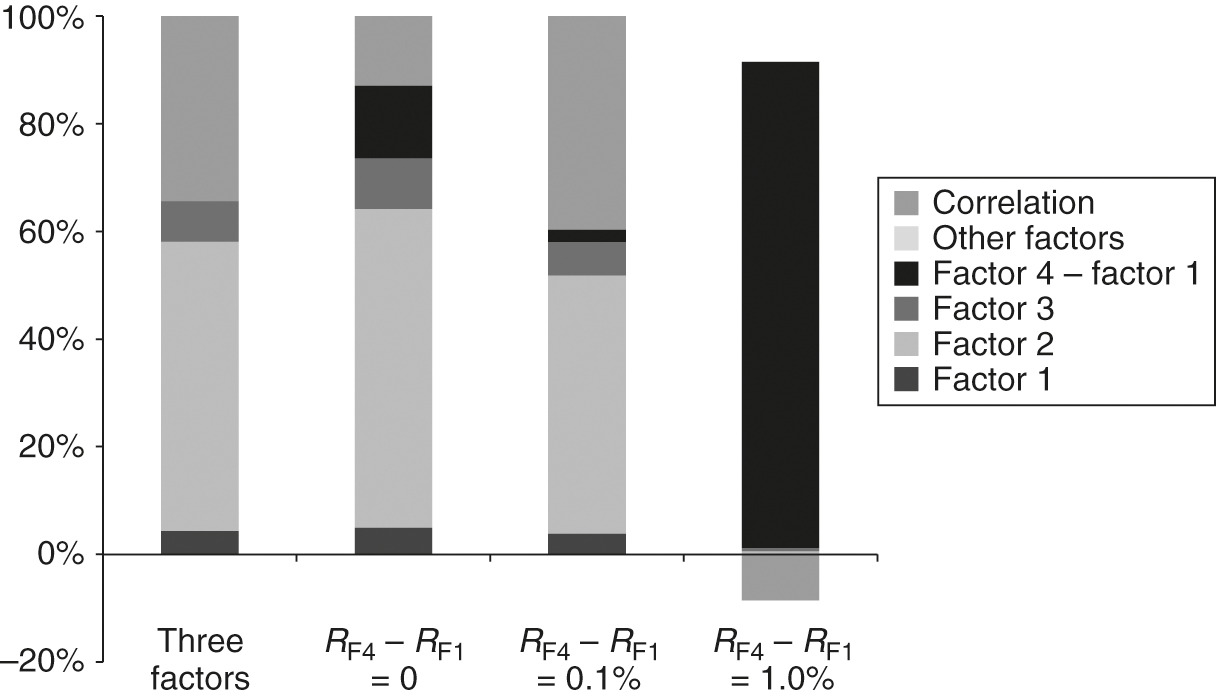
From the factor exposures and the stock volatilities and correlations in Table 3, we can decompose the variance of each optimal portfolio into (i) the contribution from each of the three factor portfolios, (ii) the contribution from the correlation of those factors, and (iii) the difference between them, which is essentially an exposure to other factors orthogonal to the three factors considered here.

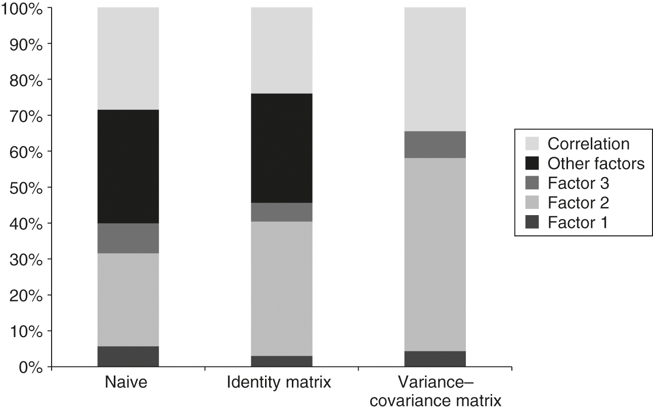
The first two approaches result in portfolios with a large component of risk derived from exposures to other factors, which have zero expected returns because they are orthogonal to the three factors considered. That is a nondesirable property of these approaches. The third approach, in which consistency is imposed by using in (2.5), has no exposure to orthogonal risk factors: the portfolio risk budget is used sensibly, ie, either for exposure to factors with a positive return or for diversification.
2.6 Adding a correlated factor
To test for robustness, we add a factor 4, which is highly correlated with factor 1. The difference between factors 4 and 1 is represented by , a long–short portfolio invested in stock 1 and short-selling stock 2 by just 1%.
| Factor 1 | Factor 2 | Factor 3 | Factor 4 | ||
|---|---|---|---|---|---|
| (%) | (%) | (%) | (%) | (%) | |
| Stock 1 | 20 | 20 | 20 | 21 | 1 |
| Stock 2 | 20 | 20 | 20 | 19 | 1 |
| Stock 3 | 20 | 20 | 20 | 20 | 0 |
| Stock 4 | 20 | 20 | 20 | 20 | 0 |
| Stock 5 | 20 | 20 | 20 | 20 | 0 |
| Stock 6 | 20 | 20 | 20 | 20 | 0 |
| Stock 7 | 20 | 20 | 20 | 20 | 0 |
| Stock 8 | 20 | 20 | 20 | 20 | 0 |
| Stock 9 | 20 | 20 | 20 | 20 | 0 |
| Stock 10 | 20 | 20 | 20 | 20 | 0 |
In addition to the expected factor returns in Table 1, we consider different assumptions for the return to factor 4. First, the return to factor 4 equals the return to factor 1. Second, stock 1 outperforms stock 2 by 10%, ie, the return to factor 4 exceeds the return to factor 1 by 0.1%. Third, stock 1 outperforms stock 2 by 100%, ie, the return to factor 4 exceeds the return to factor 1 by 1.0%.
2.6.1 Impact on expected stock returns of adding a correlated factor
We shall now investigate how this correlated factor affects the expected stock returns, the optimal portfolios and their respective variance decomposition. We start by looking at the impact on the expected stock returns.
Expected stock returns with naive approach.
In Table 7, we show that for the naive approach the magnitude of the outperformance of factor 4 over factor 1 has almost no impact on the expected stock returns. The weight of factor 1 is simply multiplied by two in the expectations. However, if instead of factor 4 we added a factor directly, then the expected stock returns would have been modified.
| Four factors | ||||
| Three | ||||
| factors | ||||
| Stock 1 | 9.03 | 11.81 | 11.83 | 12.02 |
| Stock 2 | 9.03 | 11.55 | 11.57 | 11.74 |
| Stock 3 | 3.74 | 1.09 | 1.07 | 0.89 |
| Stock 4 | 1.50 | 4.14 | 4.16 | 4.34 |
| Stock 5 | 3.80 | 6.45 | 6.47 | 6.65 |
| Stock 6 | 3.74 | 1.09 | 1.07 | 0.89 |
| Stock 7 | 1.50 | 4.14 | 4.16 | 4.34 |
| Stock 8 | 3.80 | 6.45 | 6.47 | 6.65 |
| Stock 9 | 9.03 | 11.68 | 11.70 | 11.88 |
| Stock 10 | 9.03 | 11.68 | 11.70 | 11.88 |
Expected stock returns with identity matrix.
The results are more satisfactory when the identity matrix is used because the new factor does not change the return expectations for stocks 3–10 but rather adjusts the expected returns to stocks 1 and 2 accordingly so that their return difference is consistent with that implied by the expected return for .
Expected stock returns with variance–covariance matrix.
The expected returns are more difficult to interpret. The imposed wider outperformance of stock 1 over stock 2 is easy to spot in the third and fourth cases. In the second case, it is also easy to see the consistency from stipulating that stocks 1 and 2 have the same expected return if the difference in the returns of factors 4 and 1 is zero. In each case, the returns to other stocks are adjusted so as not to deviate too strongly from the expected return for stock 1.
| Four factors | ||||
| Three | ||||
| factors | ||||
| Stock 1 | 16.13 | 16.13 | 21.13 | 66.13 |
| Stock 2 | 16.13 | 16.13 | 11.13 | 33.87 |
| Stock 3 | 7.64 | 7.64 | 7.64 | 7.64 |
| Stock 4 | 0.64 | 0.64 | 0.64 | 0.64 |
| Stock 5 | 7.84 | 7.84 | 7.84 | 7.84 |
| Stock 6 | 7.64 | 7.64 | 7.64 | 7.64 |
| Stock 7 | 0.64 | 0.64 | 0.64 | 0.64 |
| Stock 8 | 7.84 | 7.84 | 7.84 | 7.84 |
| Stock 9 | 16.13 | 16.13 | 16.13 | 16.13 |
| Stock 10 | 16.13 | 16.13 | 16.13 | 16.13 |
| Four factors | ||||
| Three | ||||
| factors | ||||
| Stock 1 | 20.60 | 13.46 | 23.39 | 112.74 |
| Stock 2 | 13.41 | 13.46 | 13.39 | 12.74 |
| Stock 3 | 9.16 | 6.87 | 10.06 | 38.79 |
| Stock 4 | 1.05 | 1.44 | 2.03 | 33.29 |
| Stock 5 | 8.54 | 5.90 | 9.57 | 42.69 |
| Stock 6 | 5.15 | 7.66 | 4.16 | 27.31 |
| Stock 7 | 0.74 | 1.98 | 1.80 | 35.80 |
| Stock 8 | 6.17 | 9.04 | 5.05 | 30.80 |
| Stock 9 | 20.07 | 24.41 | 18.37 | 35.95 |
| Stock 10 | 11.41 | 13.94 | 10.42 | 21.23 |
2.6.2 Impact of adding a correlated factor to optimal portfolios
Let us look at the mean–variance optimal portfolios generated from the expected stock returns when the correlated factor is included.
Optimal portfolios with the naive approach.
The addition of a correlated factor has a small impact on the optimal portfolios. Changing the expected outperformance of factor 4 over factor 1 also has little effect, reflecting the inconsistency between factors and expected stock returns.
| Four factors | ||||
| Three | ||||
| factors | ||||
| Stock 1 | 4.66 | 4.73 | 4.72 | 4.72 |
| Stock 2 | 36.63 | 33.90 | 33.87 | 33.64 |
| Stock 3 | 2.05 | 1.65 | 1.67 | 1.86 |
| Stock 4 | 6.80 | 12.46 | 12.49 | 12.74 |
| Stock 5 | 6.27 | 6.36 | 6.36 | 6.34 |
| Stock 6 | 17.31 | 2.97 | 2.89 | 2.14 |
| Stock 7 | 0.98 | 0.63 | 0.64 | 0.72 |
| Stock 8 | 7.46 | 11.21 | 11.23 | 11.39 |
| Stock 9 | 9.95 | 8.57 | 8.56 | 8.46 |
| Stock 10 | 40.99 | 43.22 | 43.22 | 43.21 |
| Sum | 7.74 | 3.12 | 3.09 | 2.86 |
Indeed, the larger difference in expected returns between factors 4 and 1 barely changes the model portfolio, even when this difference increases to 1%. Finally, as seen in Table 7, comparable expected returns for stocks 1 and 2 lead to a positive and larger weight in stock 2, the least volatile of the two.
Optimal portfolios with the identity matrix.
As shown in Table 11, nothing changes when factors 4 and 1 have the same expected returns. When the returns for stocks 1 and 2 are the same, the portfolio puts more weight in stock 2, the least volatile of the two. However, as the difference in returns between the two factors increases (as shown in Table 8), the increasingly large difference between the expected returns for stocks 1 and 2 translates into a greater difference in portfolio weights now favorable to stock 1.
| Four factors | ||||
| Three | ||||
| factors | ||||
| Stock 1 | 4.08 | 4.08 | 18.37 | 46.49 |
| Stock 2 | 36.47 | 36.47 | 1.08 | 74.09 |
| Stock 3 | 2.87 | 2.87 | 4.76 | 4.30 |
| Stock 4 | 2.06 | 2.06 | 4.38 | 5.11 |
| Stock 5 | 7.65 | 7.65 | 9.77 | 5.36 |
| Stock 6 | 18.99 | 18.99 | 19.36 | 3.11 |
| Stock 7 | 2.05 | 2.05 | 2.49 | 1.18 |
| Stock 8 | 8.14 | 8.14 | 8.11 | 0.95 |
| Stock 9 | 10.14 | 10.14 | 9.82 | 0.56 |
| Stock 10 | 39.34 | 39.34 | 42.44 | 11.34 |
| Sum | 9.31 | 9.31 | 21.41 | 26.48 |
Optimal portfolios with the variance–covariance matrix.
As discussed in Section 2.4, in this case the optimal mean–variance portfolio, , is proportional to a weighted average of all factor portfolios, , as implied by (2.5). The weights of each factor portfolio are given by , where the matrix is now the variance–covariance of the factor portfolios. This is a mean–variance optimization in the space of factor returns and factor variance–covariance that determines the optimal weight of each factor portfolio in the final optimal stock portfolio. It is thus not surprising that with three factors stocks 1 and 2 have the same weight since they have the same weights in factors 1, 2 and 3. When factor 4 is introduced and factors 1 and 4 have the same expected return, the factor allocation is strongly tilted in favor of the less volatile factor 1 and turns negative against the almost identical but more volatile factor 4. This explains the large overweightedness of stock 2 compared with stock 1. However, in the case where factor 4 has a higher expected return than factor 1, the optimal factor allocation will increasingly arbitrage factor 4 in favor of factor 1 as the difference in the factor returns increases. This explains the increasing difference in the weight of stock 1 with regard to the weight of stock 2.
| Four factors | ||||
| Three | ||||
| factors | ||||
| Stock 1 | 12.92 | 4.96 | 19.84 | 51.30 |
| Stock 2 | 12.92 | 32.60 | 4.36 | 55.52 |
| Stock 3 | 8.50 | 9.10 | 7.95 | 1.44 |
| Stock 4 | 2.64 | 2.52 | 2.60 | 0.44 |
| Stock 5 | 7.07 | 7.23 | 6.75 | 0.23 |
| Stock 6 | 8.50 | 9.10 | 7.95 | 1.44 |
| Stock 7 | 2.64 | 2.52 | 2.60 | 0.44 |
| Stock 8 | 7.07 | 7.23 | 6.75 | 0.23 |
| Stock 9 | 12.92 | 13.82 | 12.10 | 2.11 |
| Stock 10 | 12.92 | 13.82 | 12.10 | 2.11 |
| Sum | 0.00 | 0.00 | 0.00 | 0.00 |
2.6.3 Impact of adding a correlated factor to portfolio variance decomposition
Variance decomposition with the naive approach.
In line with the portfolios in Table 10, the factor exposures of the portfolios constructed from four factors are comparable. In addition, the allocation to factor 1 increases significantly when factor 4 is added. As a consequence, the last three portfolios in Table 10 are similar: there is little difference in the risk exposures of those portfolios. A final observation is the fact that all portfolios in Figure 2 exhibit exposure to other orthogonal factors that, by definition, have zero expected returns.

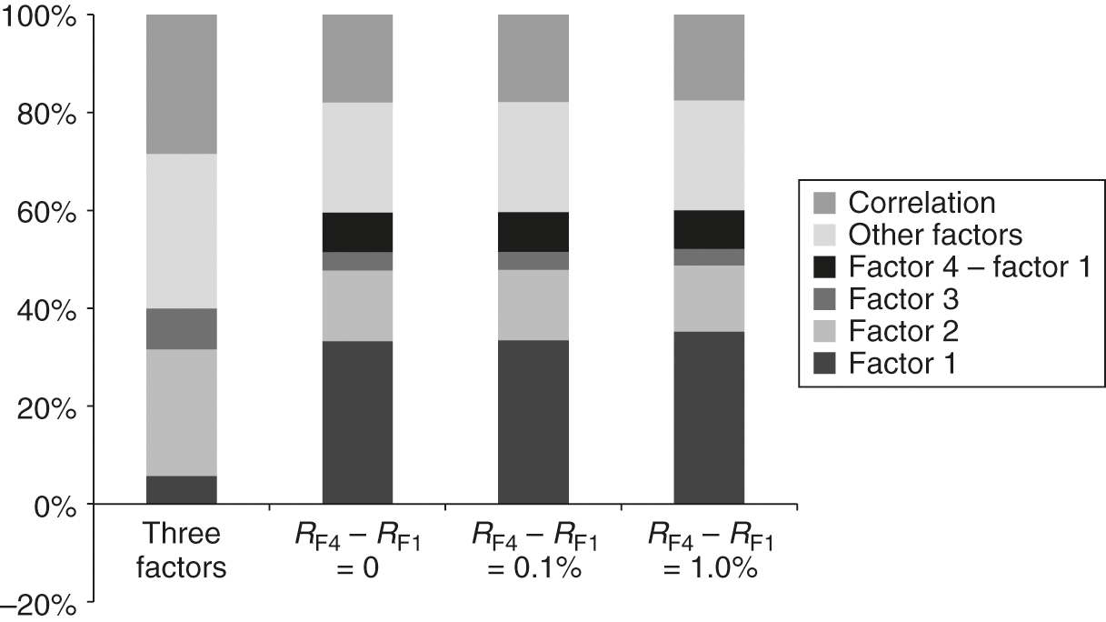
Variance decomposition with the identity matrix.
When the identity matrix is used, the factor exposures in the portfolios change significantly. In the previous case, the risk exposure to the difference between factors 4 and 1 dominated the risk of the optimal portfolio, perhaps not surprisingly. The risk-adjusted return from investing in factor 4, financed from shorting factor 1, becomes increasingly large as the difference in returns between each factor increases because the expected volatility from the difference in returns between factors 4 and 1 remains small thanks to the large correlation of their returns. The optimal portfolio is thus increasingly well positioned to capture the increasingly large risk-adjusted returns generated from shorting factor 1 to invest in factor 4. Unfortunately, all portfolios still have significant risk exposure to other factors for which the expected returns are zero.

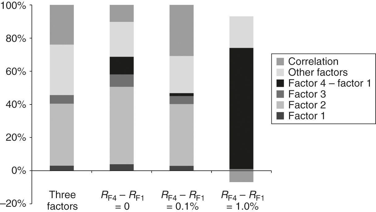
Variance decomposition with the variance–covariance matrix.
Here, the risk exposures of each portfolio are aligned with those found in Figure 3, where the identity matrix was used instead. The key difference is that no exposure to other factors can be found here, which is an important advantage of using instead of as the orthogonality measure. The portfolios are fully exposed to factors with positive expected returns and have zero exposure to factors with zero expected returns. As before, the optimal portfolio is heavily exposed to the difference between factors 4 and 1, profiting from the increasingly large risk-adjusted returns derived from the arbitrage of these two highly correlated factor portfolios.

2.7 Implications
Section 2 shows that portfolios derived from the naive approach (i) have exposures to factors orthogonal to those targeted and (ii) rely on stock returns that are inconsistent with the returns to the targeted factors. When is used as a measure of orthogonality to impose consistency between factor and stock returns, we still find a significant exposure to factors orthogonal to those considered. Moreover, such factors must have zero expected returns, which means that the risk allocation to these factors is not expected to pay. This attempt to solve for the inconsistency between factor and stock returns does not deliver portfolios that make sense. It is only when is used as a measure of orthogonality that the portfolios are fully exposed just to factors with positive expected returns. For that reason, we shall only consider this case in the remainder of our paper. Finally, we also show that, in this case, the exposure to factors in the optimal stock portfolio is determined by a mean–variance allocation to the factors based on their expected returns, volatility and correlations.
3 Factor weights and factor exposures
3.1 The general case
We shall now focus only on . As discussed in Section 2.6.2, the weights of each factor portfolio are determined by solving a mean–variance optimization problem based on the expected factor returns and the variance–covariance matrix of the factor returns. The mean–variance optimal stock allocation derived from the expected stock returns or from the expected factor returns is the same, since, from (2.5), we can write
| (3.1) |
Here, is the optimal mean–variance weight allocation to each factor, and is the same parameter used in (2.7) measuring the overall risk aversion. This can be scaled so that the ex ante volatility is set at a target level. The total risk-budget allocation is inversely proportional to the overall risk aversion.
Since factor portfolios are long–short portfolios, the optimal portfolio is also a long–short portfolio, as discussed in Section 2.4. If we use the approach to construct fully invested benchmark portfolios, then in (3.1) represents the optimal stock active weight allocation and adds to zero. The volatility of this portfolio then becomes the tracking error against the benchmark.
The risk budget allocated to a factor is by definition the factor weight times the factor volatility. It is useful to think in terms of risk-budget allocation to factors instead of weight allocation to factors, because, whereas the solution to the mean–variance factor allocation problem in terms of factor weights is a function of the leverage applied to each factor portfolio, the solution in terms of factor risk budget is invariant. This is because the volatility of the factor portfolios scales linearly with the leverage of the underlying factor long–short portfolios.
If is the vector of the mean–variance optimal risk budget allocated to each factor, is the vector of the expected information ratio for each factor and is the correlation matrix of the factor returns, then
| (3.2) |
The mapping of optimal factor risk budgets into optimal stock weights is
| (3.3) |
Equation (3.2) is the mean–variance unconstrained optimization problem of allocating to factors, rewritten in terms of risk-budget allocation to factors from factor correlations and factor information ratios, instead of the more conventional formulation in terms of factor weights from factor variance–covariance and factor returns. Equation (3.2) is invariant to changes in the volatility of factor returns, ie, invariant to the choice of leverage of the underlying factor portfolios.
Moreover, if the volatility of all factors is the same, then the expected return of each stock is equal to the multivariate beta times the expected factor return. To show this, we consider first the reverse optimization problem derived from (3.1) and (3.3):
| (3.4) |
which, using (3.2), is
| (3.5) |
As shown in the online appendix, when factors have the same volatility, the multivariate exposure of each stock to the factors is
| (3.6) |
From (3.4) and (3.5), taking into account that factors have the same volatility, the expected stock return is proportional to the multivariate beta times the expected factor return:
| (3.7) |
3.2 Maximum diversification, equal risk budget and equal risk contribution
We focused on building a robust optimal portfolio exposed to the factors we expect to pay positive returns. In order to do so – particularly when constraints apply to the portfolio – we used expected stock returns derived from the expected factor returns as optimization inputs to find the optimal stock portfolio with the desired factor exposures. The framework proposed, while robust, is sensitive to estimation errors in the factor returns. The higher the correlation of factor returns, the more likely estimation errors may cause trouble, as shown in Section 2.6.3. Therefore, we now introduce some sensible solutions that avoid the need for explicit forecasts of factor returns.
In the first example, we consider all factor information ratios to be positive and equal. In this case, the allocation to factors when the mean–variance approach is applied follows what is known as maximum diversification (MD), which was first introduced by Choueifaty and Coignard (2008).
The risk-budget allocation under MD can be derived from (3.2), assuming all of the factor information ratios are equal. When the volatility of all factors is equal, we find
| (3.8) |
where is the unit vector. Indeed, the optimal risk-budget allocation minimizes correlation, allocating higher risk budgets to factors with the lowest correlations and lower risk budgets to factors that are more correlated with others. In turn, if all factor information ratios are equal, then, when the volatility of all factors is equal, the factor returns are also equal. From (3.7), we find the expected stock returns:
| (3.9) |
For MD, the risk budget allocated to a factor can be negative even if its expected return is positive. By construction, the MD approach, when unconstrained, generates the same active univariate exposures for all factors, a result of the underlying assumption that the information ratio of all factors is equal.
The equal risk budget (ERB) simplification assumes that the risk-budget allocation to all factors is the same:
| (3.10) |
The ERB is mean–variance efficient when all factor correlations are zero and information ratios equal. From (3.4) and (3.10), the expected stock returns are
| (3.11) |
Under the ERB simplification, the risk budget allocated to each factor is always positive, but the factor exposures can be negative. Because all factor portfolios have the same volatility, the weight allocated to each factor is the same.
A third approach that falls somewhere between the two above is to allocate a risk budget to each factor so that their contribution to the risk is the same. We call this equal risk contribution (ERC), an idea that was first proposed by Maillard et al (2010). The solution is no longer mean–variance efficient for any simple choice of factor information ratios and correlations. However, it nevertheless constitutes a practical alternative approach for allocating to factors. Both the factor risk budget and the factor exposures are now positive. Since the factor volatilities are equal, the targeted ERC factor-risk-budget allocation can be numerically solved using
| (3.12) |
with the constraint that all risk budgets are positive. Once the factor risk budgets are found numerically, the optimal unconstrained stock allocation can be found from (3.3). The underlying expected stock returns can be calculated from the stock portfolio in (3.1) using reverse optimization:
| (3.13) |
By construction, and since the factor volatilities are equal, the weight of each factor is such that the product of the weight of each factor by the respective portfolio univariate exposure to the factor is equal for all factors.
In Table 13, we give the most important properties of the different choices to simplify the problem of allocating to factors.
| MD | ERB | ERC | |
|---|---|---|---|
| Factor weight | Positive or negative | Positive and equal | (Factor weight |
| for all factors | factor exposure) | ||
| Equal for all factors | |||
| Univariate factor | Positive and equal | Positive or negative | Positive |
| exposure | for all factors |
4 Application to constrained multifactor portfolios
| Active stock weights | ||||||||||||||||
| Factors | Long–short | |||||||||||||||
| factor portfolios | MD | ERB | ERC | |||||||||||||
| Market | Price- | Gross | Asset | 12M– | ||||||||||||
| Company | GICS | weight | to- | margin | growth | 1M | HML | RMW | CMA | MOM | UC | LO | UC | LO | UC | LO |
| name | sector | (%) | book | (%) | (%) | (%) | (%) | (%) | (%) | (%) | (%) | (%) | (%) | (%) | (%) | (%) |
| Adidas AG | CD | 1.4 | 4.7 | 47 | 14 | 24 | 2.1 | 3.2 | 2.6 | 3.1 | 1.9 | 2.5 | 0.8 | 1.2 | 1.1 | 0.2 |
| LVMH Moet | CD | 2.5 | 3.5 | 65 | 3 | 66 | 0.0 | 3.2 | 2.6 | 3.1 | 3.7 | 5.0 | 4.0 | 5.0 | 4.0 | 5.0 |
| Hennessy Louis | ||||||||||||||||
| Vuitton SE | ||||||||||||||||
| Vivendi SA | CD | 0.9 | 1.3 | 37 | 7 | 23 | 0.0 | 0.0 | 2.6 | 0.0 | 0.1 | 0.9 | 1.1 | 0.1 | 0.9 | 0.9 |
| Volkswagen AG | CD | 1.1 | 0.8 | 19 | 7 | 12 | 2.1 | 3.2 | 0.0 | 3.1 | 2.1 | 1.1 | 1.9 | 1.1 | 2.0 | 1.1 |
| Pref | ||||||||||||||||
| Daimler AG | CD | 2.7 | 1.3 | 21 | 12 | 15 | 0.0 | 3.2 | 0.0 | 0.0 | 2.0 | 2.7 | 1.4 | 2.7 | 1.7 | 2.7 |
| Bayerische | CD | 1.1 | 1.2 | 24 | 9 | 15 | 2.1 | 0.0 | 0.0 | 0.0 | 1.5 | 1.6 | 0.9 | 0.0 | 1.0 | 0.6 |
| Motoren | ||||||||||||||||
| Werke AG | ||||||||||||||||
| Industria de | CD | 1.6 | 7.5 | 28 | 13 | 15 | 2.1 | 0.0 | 2.6 | 3.1 | 3.2 | 1.6 | 3.4 | 1.6 | 3.3 | 1.6 |
| Diseno Textil, | ||||||||||||||||
| SA | ||||||||||||||||
| L’Oreal SA | CS | 1.9 | 4.0 | 72 | 6 | 10 | 2.1 | 3.2 | 2.6 | 3.1 | 2.2 | 5.0 | 3.0 | 5.0 | 2.9 | 5.0 |
| Anheuser-Busch | CS | 3.1 | 2.9 | 58 | 98 | 10 | 0.0 | 3.2 | 2.6 | 3.1 | 0.3 | 3.1 | 1.1 | 3.1 | 0.6 | 3.1 |
| InBev SA/NV | ||||||||||||||||
| Royal Ahold | CS | 0.9 | 1.6 | 27 | 133 | 19 | 2.1 | 3.2 | 2.6 | 3.1 | 2.2 | 0.9 | 3.0 | 0.9 | 2.9 | 0.9 |
| Delhaize NV | ||||||||||||||||
| Danone SA | CS | 1.7 | 2.8 | 51 | 36 | 6 | 2.1 | 0.0 | 0.0 | 0.0 | 1.5 | 1.7 | 0.9 | 1.7 | 1.0 | 1.7 |
| Unilever NV | CS | 3.3 | 6.8 | 43 | 8 | 23 | 2.1 | 3.2 | 2.6 | 3.1 | 1.8 | 3.3 | 0.2 | 3.3 | 0.4 | 3.3 |
| Cert Shs | ||||||||||||||||
| Total SA | EN | 4.5 | 1.3 | 24 | 6 | 8 | 2.1 | 3.2 | 2.6 | 3.1 | 2.1 | 4.5 | 2.1 | 4.5 | 2.2 | 4.5 |
| Eni SpA | EN | 1.4 | 1.1 | 36 | 11 | 1 | 2.1 | 3.2 | 2.6 | 3.1 | 2.1 | 4.4 | 2.1 | 5.0 | 2.2 | 5.0 |
| Intesa Sanpaolo | FN | 1.8 | 0.9 | NA | 7 | 43 | 0.0 | 0.0 | 2.6 | 0.0 | 0.1 | 1.8 | 1.1 | 1.8 | 0.9 | 1.8 |
| SpA | ||||||||||||||||
| Allianz SE | FN | 3.5 | 1.1 | NA | 4 | 44 | 2.1 | 0.0 | 2.6 | 0.0 | 1.6 | 3.5 | 2.0 | 3.5 | 1.9 | 3.5 |
| Munich | FN | 1.2 | 0.9 | NA | 0 | 27 | 0.0 | 0.0 | 0.0 | 3.1 | 1.6 | 1.2 | 1.4 | 1.2 | 1.4 | 1.2 |
| Reinsurance | ||||||||||||||||
| Company | ||||||||||||||||
| Banco Bilbao | FN | 2.1 | 0.9 | NA | 3 | 43 | 0.0 | 0.0 | 2.6 | 0.0 | 0.1 | 2.1 | 1.1 | 2.1 | 0.9 | 2.1 |
| Vizcaya | ||||||||||||||||
| Argentaria, SA | ||||||||||||||||
| Banco Santander | FN | 3.9 | 0.8 | NA | 0 | 55 | 2.1 | 0.0 | 2.6 | 3.1 | 3.2 | 5.0 | 3.4 | 5.0 | 3.3 | 5.0 |
| SA | ||||||||||||||||
| Deutsche Bank | FN | 1.2 | 0.4 | NA | 2 | 29 | 2.1 | 0.0 | 2.6 | 3.1 | 0.1 | 1.2 | 0.7 | 1.2 | 0.5 | 1.2 |
| AG | ||||||||||||||||
| Société Générale | FN | 1.6 | 0.6 | NA | 4 | 60 | 2.1 | 0.0 | 0.0 | 3.1 | 3.1 | 4.2 | 2.3 | 4.4 | 2.4 | 5.0 |
| SA Class A | ||||||||||||||||
| AXA SA | FN | 2.2 | 1.0 | NA | 1 | 40 | 2.1 | 0.0 | 0.0 | 3.1 | 3.1 | 2.2 | 2.3 | 2.2 | 2.4 | 2.2 |
| ING Groep NV | FN | 2.6 | 1.0 | NA | 16 | 55 | 2.1 | 0.0 | 2.6 | 3.1 | 0.2 | 2.6 | 1.6 | 1.6 | 1.2 | 0.1 |
| BNP Paribas | FN | 3.0 | 0.7 | NA | 4 | 48 | 2.1 | 0.0 | 2.6 | 3.1 | 2.9 | 4.0 | 1.2 | 3.0 | 1.5 | 3.0 |
| SA Class A | ||||||||||||||||
| Unibail-Rodamco | FN | 0.9 | 1.3 | 88 | 7 | 1 | 2.1 | 0.0 | 2.6 | 3.1 | 3.2 | 0.9 | 3.4 | 0.9 | 3.3 | 0.9 |
| SE | ||||||||||||||||
| Fresenius SE & | HC | 1.3 | 3.2 | 32 | 8 | 17 | 0.0 | 3.2 | 0.0 | 0.0 | 2.0 | 1.3 | 1.4 | 1.3 | 1.7 | 1.3 |
| Co. KGaA | ||||||||||||||||
| Bayer AG | HC | 3.9 | 2.7 | 57 | 10 | 36 | 0.0 | 0.0 | 0.0 | 3.1 | 1.6 | 4.6 | 1.4 | 3.5 | 1.4 | 5.0 |
| Sanofi | HC | 4.0 | 1.7 | 64 | 2 | 19 | 2.1 | 3.2 | 2.6 | 0.0 | 3.6 | 5.0 | 3.5 | 5.0 | 3.6 | 5.0 |
| Essilor | HC | 1.1 | 3.5 | 59 | 10 | 2 | 2.1 | 0.0 | 2.6 | 3.1 | 3.2 | 1.1 | 3.4 | 1.1 | 3.3 | 1.1 |
| International SA | ||||||||||||||||
| Airbus SE | ID | 1.7 | 13.3 | 8 | 5 | 50 | 2.1 | 3.2 | 2.6 | 3.1 | 2.1 | 1.7 | 2.1 | 1.7 | 2.2 | 1.7 |
| Safran SA | ID | 1.2 | 4.4 | 23 | 8 | 37 | 2.1 | 3.2 | 2.6 | 3.1 | 2.1 | 1.2 | 2.1 | 1.2 | 2.2 | 1.2 |
| Deutsche Post | ID | 1.4 | 3.4 | 44 | 1 | 30 | 2.1 | 3.2 | 2.6 | 3.1 | 0.9 | 1.4 | 0.3 | 1.4 | 0.1 | 1.4 |
| AG | ||||||||||||||||
| VINCI SA | ID | 1.8 | 2.2 | 13 | 9 | 22 | 0.0 | 3.2 | 2.6 | 3.1 | 3.7 | 1.8 | 4.0 | 1.8 | 4.0 | 1.8 |
| Schneider | ID | 1.6 | 1.8 | 38 | 2 | 28 | 2.1 | 3.2 | 2.6 | 3.1 | 2.1 | 3.1 | 2.1 | 5.0 | 2.2 | 5.0 |
| Electric SE | ||||||||||||||||
| Siemens AG | ID | 4.2 | 2.5 | 30 | 4 | 36 | 0.0 | 0.0 | 0.0 | 0.0 | 0.0 | 4.2 | 0.0 | 4.2 | 0.0 | 4.2 |
| Royal Philips | ID | 1.2 | 2.1 | 43 | 5 | 42 | 2.1 | 3.2 | 0.0 | 3.1 | 5.1 | 5.0 | 3.7 | 5.0 | 4.1 | 5.0 |
| NV | ||||||||||||||||
| Compagnie de | ID | 1.0 | 1.3 | 26 | 2 | 36 | 2.1 | 0.0 | 2.6 | 0.0 | 1.6 | 1.0 | 2.0 | 5.0 | 1.9 | 5.0 |
| Saint-Gobain SA | ||||||||||||||||
| SAP SE | IT | 3.8 | 3.8 | 72 | 7 | 27 | 0.0 | 3.2 | 2.6 | 3.1 | 3.7 | 5.0 | 4.0 | 5.0 | 4.0 | 5.0 |
| Nokia Oyj | IT | 1.3 | 1.3 | 36 | 114 | 12 | 2.1 | 3.2 | 2.6 | 3.1 | 2.2 | 1.3 | 3.0 | 1.3 | 2.9 | 1.3 |
| ASML Holding | IT | 2.1 | 4.7 | 43 | 29 | 26 | 2.1 | 0.0 | 0.0 | 0.0 | 1.5 | 2.1 | 0.9 | 2.1 | 1.0 | 2.1 |
| NV | ||||||||||||||||
| Air Liquide SA | MA | 1.8 | 2.5 | 36 | 53 | 23 | 0.0 | 3.2 | 2.6 | 0.0 | 1.9 | 2.3 | 0.3 | 1.8 | 0.8 | 1.8 |
| CRH Plc | MA | 1.1 | 2.0 | 33 | 1 | 22 | 2.1 | 0.0 | 2.6 | 3.1 | 0.1 | 1.1 | 0.7 | 1.1 | 0.5 | 1.1 |
| BASF SE | MA | 3.2 | 2.6 | 31 | 7 | 23 | 2.1 | 3.2 | 0.0 | 3.1 | 1.9 | 3.2 | 1.0 | 3.2 | 1.3 | 3.2 |
| Orange SA | TS | 1.2 | 1.5 | 58 | 4 | 4 | 2.1 | 3.2 | 2.6 | 3.1 | 1.8 | 4.2 | 0.2 | 1.2 | 0.4 | 1.2 |
| Telefonica SA | TS | 1.8 | 2.4 | 16 | 3 | 12 | 0.0 | 3.2 | 0.0 | 0.0 | 2.0 | 1.8 | 1.4 | 1.8 | 1.7 | 1.8 |
| Deutsche | TS | 2.1 | 2.6 | 35 | 3 | 13 | 2.1 | 0.0 | 2.6 | 3.1 | 0.2 | 2.1 | 1.6 | 5.0 | 1.2 | 3.6 |
| Telekom AG | ||||||||||||||||
| E.ON SE | UT | 0.8 | 1.1 | 7 | 43 | 10 | 0.0 | 3.2 | 2.6 | 0.0 | 1.9 | 0.8 | 0.3 | 0.8 | 0.8 | 0.8 |
| Enel SpA | UT | 1.6 | 1.2 | 49 | 3 | 24 | 2.1 | 3.2 | 0.0 | 3.1 | 2.1 | 3.0 | 1.9 | 5.0 | 2.0 | 5.0 |
| ENGIE SA | UT | 1.0 | 0.7 | 23 | 1 | 1 | 2.1 | 0.0 | 0.0 | 3.1 | 0.1 | 1.0 | 0.5 | 1.0 | 0.4 | 1.0 |
| Iberdrola SA | UT | 1.7 | 1.0 | 19 | 2 | 17 | 0.0 | 0.0 | 2.6 | 0.0 | 0.1 | 1.7 | 1.1 | 1.7 | 0.9 | 1.7 |
Let us consider an example. The objective is to construct a fully invested equity multifactor portfolio where the tracking error relative to the benchmark index derives from the active factor exposures. For this reason, we shall consider as the zero-sum portfolio with optimal active stock weights, the volatility of which is the tracking error risk of the benchmarked portfolio. If we add the benchmark index to , we find the optimal stock weights in the fully invested benchmarked portfolio, ie, with stock weights totaling 100%.
We consider the unconstrained case, where the portfolio may include short positions. This is the case if the size of the short of a given stock in exceeds the weight of the stock in the benchmark portfolio. For this reason, we also include the case of the long-only constrained, fully invested portfolio, where no short positions are allowed. This portfolio can be obtained numerically by solving (3.1) under long-only constraints from the vector of expected stock returns ; this can be obtained from (3.13) in both the general case and the ERC case and simplifies to (3.9) and (3.11) in the MD and ERB cases, respectively.
In this example, we use the Stoxx 50 index on July 21, 2017 and construct factor portfolios using four known factors: HML, RMW and CMA, from the factor model proposed by Fama and French (2015), and MOM, a factor proposed by Carhart (1997). The first three use price-to-book, gross profit and asset growth as indicators. The last uses the historical returns of stocks over eleven months, calculated one month before the date of portfolio construction. We shall consider the three cases of active factor allocation discussed above, that is, MD, ERB and ERC.
In Table 14, we show the company names of the stocks in the Stoxx 50 index, organized by sector. CD stands for consumer discretionary, CS for consumer staples, EN for energy, FN for financials, HC for health care, ID for industrials, IT for information technology, MA for materials, TS for telecommunication services and UT for utilities. We did not separate real estate from financials as is the case in recent Global Industry Classification Standard (GICS) definitions. We also include the price-to-book used to construct the HML factor, the gross margin used for RMW, the asset growth used for CMA and the eleven-month stock returns calculated one month prior to the portfolio formation for MOM. In the columns titled “Long–short factor portfolios”, we show how the long–short factor portfolios were constructed from the factor data. We enforced sector neutrality. Thus, in each sector, we allocated a positive weight to about one-third of the stocks ranked the highest for each respective factor, and we allocated a negative weight to about one-third of the stocks ranked lowest for each respective factor. Each long–short factor portfolio is cash neutral and stocks are equally weighted. RMW does not apply to financials. For HML, the price-to-book of stocks is ranked from the cheapest as the lowest to the most expensive as the highest. Similarly, for CMA, stocks with lower asset growth are preferred. For RMW and MOM, higher values of gross margin are preferred and a higher performance of stocks is preferred, respectively.
The is calculated from three years of history of weekly stock returns and used to find the leverage required to set the ex ante volatility of each long–short portfolio to 3%. We also calculated the factor correlation matrix using historical data and the long–short factor portfolios . In our example, this posed no problem and the matrix could be inverted when used in (3.1) to solve for the optimization problem. However, in real applications we recommend that is estimated either from a Bayesian approach, eg, as proposed by Ledoit and Wolf (2004), or from a risk model, eg, based on dimensionality reduction via principal components analysis. Otherwise, as the number of assets grows, it is likely that the estimation errors become too large and cannot be inverted in (3.1).
Using these long–short portfolios, we then followed the approach described in Section 3 and calculated the factor risk budgets for the three cases. The information ratio of all factors was set to 0.5 and was set to 1. We used (3.8) for MD and (3.10) for ERB. For ERC, we numerically solved (3.12). For details on how to numerically solve for the factor risk budgets so that the contribution of each factor toward the total volatility of the multifactor long–short portfolio aggregation can be found, see Maillard et al (2010) and Leote de Carvalho et al (2012).
The factor risk budgets obtained can be found in Table 15. Here, we include a column with factor weights for the unconstrained portfolio and two for the univariate factor active exposures, the first for the unconstrained portfolio and the second for the long-only constrained portfolio.
| MD | ERB | ERC | |||||||
| Exposure | Exposure | Exposure | |||||||
| Weight | Weight | Weight | |||||||
| UC | UC | LO | UC | UC | LO | UC | UC | LO | |
| Factors | (%) | (%) | (%) | (%) | (%) | (%) | (%) | (%) | (%) |
| HML | 73 | 53 | 37 | 44 | 50 | 29 | 51 | 49 | 29 |
| RMW | 62 | 53 | 58 | 44 | 42 | 52 | 52 | 48 | 51 |
| CMA | 5 | 53 | 35 | 44 | 77 | 47 | 35 | 71 | 43 |
| MOM | 50 | 53 | 44 | 44 | 57 | 30 | 45 | 56 | 32 |
The vector with the risk budget of each factor is then used in (3.2) along with the matrix to calculate the unconstrained optimal stock active weights shown in Table 14. The constrained portfolios are calculated numerically from (3.1), from the variance–covariance matrix and the expected stock returns , under the imposition that the sum of stock active weights must be zero and that no short or leveraged positions are allowed for any stock. For this, the expected returns are calculated first using (3.9), (3.11) and (3.13) for MD, ERB and ERC, respectively. The expected stock returns for the MD and ERB cases are given in Table 16 along with the univariate and multivariate betas. It is clear that they follow from (3.9) and (3.11), respectively.
| Stock | |||||||||||
| Factor exposure | Factor exposure | excess | |||||||||
| multivariate | univariate | returns | |||||||||
| GICS | HML | RMW | CMA | MOM | HML | RMW | CMA | MOM | MD | ERB | |
| Company name | sector | (%) | (%) | (%) | (%) | (%) | (%) | (%) | (%) | (%) | (%) |
| Adidas AG | CD | 103 | 90 | 192 | 237 | 46 | 106 | 85 | 195 | 3.6 | 2.6 |
| LVMH Moet Hennessy | CD | 42 | 53 | 205 | 84 | 120 | 60 | 246 | 136 | 5.8 | 8.4 |
| Louis Vuitton SE | |||||||||||
| Vivendi SA | CD | 36 | 109 | 210 | 23 | 93 | 94 | 196 | 56 | 1.3 | 3.8 |
| Volkswagen AG Pref | CD | 339 | 535 | 403 | 231 | 704 | 659 | 514 | 279 | 0.4 | 4.2 |
| Daimler AG | CD | 103 | 323 | 245 | 37 | 302 | 340 | 303 | 22 | 0.9 | 4.3 |
| Bayerische Motoren | CD | 258 | 303 | 198 | 66 | 424 | 353 | 340 | 24 | 3.3 | 6.5 |
| Werke AG | |||||||||||
| Industria de Diseno | CD | 38 | 43 | 52 | 11 | 74 | 51 | 73 | 10 | 0.9 | 1.6 |
| Textil, SA | |||||||||||
| L’Oreal SA | CS | 142 | 39 | 161 | 60 | 59 | 9 | 104 | 108 | 0.6 | 2.4 |
| Anheuser-Busch | CS | 76 | 31 | 41 | 111 | 34 | 32 | 23 | 98 | 2.7 | 2.8 |
| InBev SA/NV | |||||||||||
| Royal Ahold Delhaize | CS | 138 | 117 | 150 | 28 | 95 | 157 | 89 | 102 | 2.4 | 3.8 |
| NV | |||||||||||
| Danone SA | CS | 16 | 47 | 60 | 61 | 18 | 32 | 66 | 68 | 0.9 | 1.8 |
| Unilever NV Cert Shs | CS | 255 | 201 | 156 | 76 | 136 | 121 | 44 | 108 | 3.4 | 1.6 |
| Total SA | EN | 17 | 146 | 196 | 84 | 108 | 125 | 206 | 105 | 1.8 | 4.4 |
| Eni SpA | EN | 119 | 93 | 209 | 46 | 240 | 112 | 278 | 62 | 4.2 | 7.0 |
| Intesa Sanpaolo SpA | FN | 586 | 32 | 88 | 306 | 512 | 123 | 277 | 205 | 11.6 | 13.1 |
| Allianz SE | FN | 40 | 151 | 167 | 35 | 157 | 153 | 194 | 41 | 1.4 | 3.6 |
| Munich Reinsurance | FN | 21 | 38 | 98 | 22 | 82 | 47 | 103 | 9 | 0.9 | 1.9 |
| Company | |||||||||||
| Banco Bilbao | FN | 415 | 82 | 218 | 330 | 502 | 124 | 502 | 313 | 13.2 | 17.9 |
| Vizcaya Argentaria, SA | |||||||||||
| Banco Santander SA | FN | 460 | 102 | 320 | 298 | 608 | 159 | 619 | 295 | 14.6 | 20.4 |
| Deutsche Bank AG | FN | 573 | 233 | 268 | 162 | 745 | 345 | 590 | 108 | 11.5 | 16.5 |
| Société Générale | FN | 673 | 98 | 52 | 433 | 669 | 187 | 489 | 341 | 15.9 | 19.7 |
| SA Class A | |||||||||||
| AXA SA | FN | 216 | 151 | 99 | 119 | 288 | 182 | 233 | 86 | 4.2 | 6.4 |
| ING Groep NV | FN | 221 | 88 | 199 | 224 | 314 | 100 | 361 | 226 | 8.3 | 12.0 |
| BNP Paribas SA | FN | 589 | 88 | 5 | 415 | 561 | 159 | 396 | 326 | 13.8 | 16.8 |
| Class A | |||||||||||
| Unibail-Rodamco SE | FN | 127 | 1 | 113 | 112 | 56 | 11 | 23 | 70 | 1.9 | 1.4 |
| Fresenius SE & Co. | HC | 148 | 152 | 74 | 66 | 64 | 126 | 16 | 58 | 4.4 | 4.0 |
| KGaA | |||||||||||
| Bayer AG | HC | 76 | 182 | 131 | 87 | 25 | 146 | 112 | 94 | 0.6 | 1.3 |
| Sanofi | HC | 33 | 19 | 208 | 28 | 136 | 7 | 219 | 20 | 3.5 | 5.7 |
| Essilor International | HC | 125 | 85 | 58 | 45 | 69 | 62 | 16 | 31 | 3.0 | 2.7 |
| SA | |||||||||||
| Airbus SE | ID | 77 | 447 | 68 | 237 | 125 | 423 | 22 | 129 | 3.0 | 2.2 |
| Safran SA | ID | 23 | 316 | 60 | 181 | 49 | 289 | 9 | 106 | 2.6 | 2.1 |
| Deutsche Post AG | ID | 113 | 78 | 333 | 45 | 79 | 54 | 265 | 33 | 1.5 | 4.8 |
| VINCI SA | ID | 71 | 71 | 33 | 9 | 73 | 90 | 0 | 38 | 0.6 | 0.8 |
| Schneider Electric | ID | 145 | 22 | 239 | 12 | 272 | 58 | 309 | 22 | 5.3 | 8.1 |
| SA | |||||||||||
| Siemens AG | ID | 147 | 105 | 114 | 71 | 221 | 128 | 203 | 59 | 3.4 | 5.3 |
| Royal Philips NV | ID | 260 | 32 | 22 | 146 | 260 | 70 | 185 | 112 | 5.9 | 7.3 |
| Compagnie de | ID | 302 | 96 | 98 | 110 | 361 | 150 | 274 | 77 | 6.2 | 8.4 |
| Saint-Gobain SA | |||||||||||
| SAP SE | IT | 20 | 20 | 122 | 37 | 81 | 17 | 140 | 59 | 2.4 | 4.0 |
| Nokia Oyj | IT | 294 | 216 | 270 | 11 | 211 | 290 | 123 | 129 | 2.7 | 5.0 |
| ASML Holding | IT | 145 | 208 | 238 | 59 | 18 | 159 | 177 | 94 | 0.9 | 2.0 |
| NV | |||||||||||
| Air Liquide SA | MA | 51 | 0 | 124 | 83 | 102 | 4 | 169 | 106 | 3.9 | 5.7 |
| CRH Plc | MA | 252 | 123 | 128 | 66 | 355 | 197 | 238 | 90 | 2.9 | 4.6 |
| BASF SE | MA | 17 | 195 | 299 | 90 | 170 | 171 | 310 | 126 | 2.7 | 6.5 |
| Orange SA | TS | 88 | 52 | 12 | 46 | 75 | 22 | 22 | 50 | 1.2 | 1.0 |
| Telefonica SA | TS | 108 | 164 | 137 | 165 | 197 | 160 | 228 | 153 | 3.7 | 6.3 |
| Deutsche | TS | 83 | 57 | 161 | 22 | 15 | 39 | 114 | 15 | 0.0 | 1.6 |
| Telekom AG | |||||||||||
| E.ON SE | UT | 154 | 336 | 580 | 10 | 219 | 290 | 502 | 103 | 1.5 | 8.0 |
| Enel SpA | UT | 33 | 23 | 49 | 107 | 50 | 11 | 91 | 110 | 2.5 | 3.6 |
| ENGIE SA | UT | 60 | 106 | 185 | 43 | 185 | 127 | 204 | 27 | 1.5 | 3.5 |
| Iberdrola SA | UT | 46 | 4 | 25 | 34 | 55 | 9 | 56 | 33 | 1.5 | 2.0 |
The objective of Table 14 is to show the optimal constrained and unconstrained multifactor portfolios. We include the weights of each stock in the market capitalization index and the active weights in each case of factor allocation considered. It is interesting to note that the cross-sectional correlation of active weights for the unconstrained and constrained portfolios in Table 14 is 80% for MD and 75% for both ERB and ERC. This demonstrates empirically that, despite the strong long-only constraint, the optimizer still delivers active weights that remain relatively close to the unconstrained case.
In Table 14, we also find that the cross-sectional correlation between the MD and ERB unconstrained portfolio active weights is 92%, between the MD and ERC unconstrained active weights is 96% and between the ERB and ERC unconstrained active weights is 99%. Compared with the figures cited in the previous paragraph, this shows that the impact of portfolio constraints on the final portfolio is stronger than the assumptions used for deciding on the risk-budget allocation to the factors. Also, for as long as factor correlations are low, we should expect ERB and ERC to be led to rather similar portfolio stock weights, as is the case in this example.
The cross-sectional correlation between the ERB and ERC constrained portfolio active weights is 99%, showing that there is hardly any difference between ERB and ERC when it comes to portfolio allocation in the constrained case either. This is not surprising, as the starting unconstrained portfolios were already very similar. In turn, the cross-sectional correlation between the MD and ERB constrained portfolio active weights is 75%, and between the MD and ERC constrained active weights is 79%. While there is little difference between choosing ERB or ERC, choosing MD leads to larger differences in the final constrained portfolios.
Finally, from Table 15 we can see to what extent the portfolio constraints pushed factor exposures away from the targeted risk budget, which gives a clear indication of the impact of constraints on factor exposures. In all three cases, we found an underexposure to HML, CMA and MOM and an overexposure to RMW in the constrained portfolios.
5 Conclusions
We discuss the question of multifactor portfolio construction and show that the simplistic approaches often used by practitioners tend to be suboptimal. We first focus on three approaches to generate expected stock returns from expected factor returns with the objective of using these as inputs in mean–variance optimization for the construction of realistic portfolios with targeted multifactor exposures. We demonstrate that the two most simplistic approaches generate portfolios with a significant percentage of the tracking error allocated to unintended exposures to factors orthogonal to those targeted. Indeed, we show that expected stock returns must be derived in a robust fashion from expected factor returns if we wish to use them in mean–variance optimization and make sure that portfolios have only exposures to targeted factors. We discuss at length the framework that we recommend for this purpose. Second, we provide a detailed example to illustrate the framework, and we demonstrate its efficacy for the construction of realistic constrained portfolios, eg, long only. We show that even when applying constraints, the portfolios retain much of the targeted factor exposures while minimizing the impact of constraints.
Building portfolios with multiple factor exposures for factor investing is certainly not easy, especially when realistic constraints apply. We believe that our paper makes an important contribution toward highlighting the problems in factor investing and proposing solutions, particularly for benchmarked constrained factor investing in equities.
Declaration of interest
The authors report no conflicts of interest. The authors alone are responsible for the content and writing of the paper.
References
- Amenc, N., Goltz, F., and Lodh, A. (2018). Mind the gap: on the importance of understanding and controlling market risk in smart beta strategies. Journal of Portfolio Management 44(4), 60–70 (https://doi.org/10.3905/jpm.2018.44.4.060).
- Basu, S. (1977). Investment performance of common stocks in relation to their price–earnings ratios: a test of the efficient market hypothesis. Journal of Finance 32(3), 663–682 (https://doi.org/10.1111/j.1540-6261.1977.tb01979.x).
- Blitz, D., Hanauer, X. H., Vidojevic, M., and van Vliet, P. (2018). Five concerns about the five-factor model. Journal of Portfolio Management 44(4), 71–78 (https://doi.org/10.3905/jpm.2018.44.4.071).
- Carhart, M. M. (1997). On persistence in mutual fund performance. Journal of Finance 52(1), 57–82 (https://doi.org/10.1111/j.1540-6261.1997.tb03808.x).
- Choueifaty, Y., and Coignard, Y. (2008). Towards maximum diversification. Journal of Portfolio Management 35(1), 40–51 (https://doi.org/10.3905/JPM.2008.35.1.40).
- Fama, E., and French, F. (2015). A five-factor asset pricing model. Journal of Financial Economics 116(1), 1–22 (https://doi.org/10.1016/j.jfineco.2014.10.010).
- Harvey, C. R., Yan, L., and Zhu, H. (2016). … and the cross-section of expected returns. Review of Financial Studies 29(1), 5–68 (https://doi.org/10.1093/rfs/hhv059).
- Haugen, R., and Baker, N. (1996). Commonality in the determinants of expected stock returns. Journal of Financial Economics 41(2), 401–439 (https://doi.org/10.1016/0304-405X(95)00868-F).
- Haugen, R., and Heines, A. J. (1972). On the evidence supporting the existence of risk premiums in the capital market. Working Paper 1783797, Social Science Research Network (https://doi.org/10.2139/ssrn.1783797).
- Hou, K., Xue, C., and Zhang, L. (2017). Replicating anomalies. Working Paper 23394, National Bureau of Economic Research. URL: https://papers.ssrn.com/sol3/papers.cfm?abstract_id=2961979.
- Jagadeesh, N., and Titman, S. (1993). Returns to buying winners and selling losers: implications for stock market efficiency. Journal of Finance 48(1), 65–91 (https://doi.org/10.1111/j.1540-6261.1993.tb04702.x).
- Ledoit, O., and Wolf, M. (2004). Honey, I shrunk the sample covariance matrix. Journal of Portfolio Management 30(4), 110–119 (https://doi.org/10.3905/jpm.2004.110).
- Leote de Carvalho, R. (2016). Cross-sectional regression equity factor models: implementation pitfalls. Working Paper, Social Science Research Network.
- Leote de Carvalho, R., Lu, X., and Moulin, P. (2012). Demystifying equity risk-based strategies: a simple alpha plus beta description. Journal of Portfolio Management 38(3), 56–70 (https://doi.org/10.3905/jpm.2012.38.3.056).
- Leote de Carvalho, R., Lu, X., and Moulin, P. (2014). An integrated risk-budgeting approach for multi-strategy equity portfolios. Journal of Asset Management 15(1), 24–47 (https://doi.org/10.1057/jam.2014.11).
- Leote de Carvalho, R., Lu, X., Soupé, F., and Dugnolle, P. (2017). Diversify and purify factor premiums in equity markets. In Factor Investing: From Traditional to Alternative Risk Premia, Jurczenko, E. (ed). Elsevier (https://doi.org/10.2139/ssrn.2894171).
- Lo, A. L., and Patel, P. N. (2008). 130/30: the new long-only. Journal of Portfolio Management 34(2), 12–38 (https://doi.org/10.3905/jpm.2008.701615).
- Maillard, S., Roncalli, T., and Teiletche, J. (2010). The properties of equally weighted risk contribution portfolios. Journal of Portfolio Management 36(4), 60–70 (https://doi.org/10.3905/jpm.2010.36.4.060).
- Novy-Marx, R. (2013). The other side of value: the gross profitability premium. Journal of Financial Economics 108(1), 1–28 (https://doi.org/10.1016/j.jfineco.2013.01.003).
- Qian, E. E., Hua, R. H., and Sorensen, E. H. (2007). Quantitative Equity Portfolio Management: Modern Techniques and Applications. Chapman & Hall/CRC Taylor Francis (https://doi.org/10.1201/9781420010794).
Only users who have a paid subscription or are part of a corporate subscription are able to print or copy content.
To access these options, along with all other subscription benefits, please contact info@risk.net or view our subscription options here: http://subscriptions.risk.net/subscribe
You are currently unable to print this content. Please contact info@risk.net to find out more.
You are currently unable to copy this content. Please contact info@risk.net to find out more.
Copyright Infopro Digital Limited. All rights reserved.
As outlined in our terms and conditions, https://www.infopro-digital.com/terms-and-conditions/subscriptions/ (point 2.4), printing is limited to a single copy.
If you would like to purchase additional rights please email info@risk.net
Copyright Infopro Digital Limited. All rights reserved.
You may share this content using our article tools. As outlined in our terms and conditions, https://www.infopro-digital.com/terms-and-conditions/subscriptions/ (clause 2.4), an Authorised User may only make one copy of the materials for their own personal use. You must also comply with the restrictions in clause 2.5.
If you would like to purchase additional rights please email info@risk.net