Hull and White on the pros and cons of expected shortfall

Expected shortfall may be a more effective prudential measure than value-at-risk, but it is almost impossible to back-test and may be less stable than its predecessor, warn John Hull and Alan White. They also propose a simple solution for the problem created by overlapping time horizons in draft trading book rules

John Hull

The Basel Committee on Banking Supervision's ongoing attempts to redraw the capital rules for trading books is likely to lead to major changes in the way market risk capital is calculated.¹ After almost 20 years of using value-at-risk measures with a 10-day time horizon and a 99% confidence level, regulators have decided it is time to rethink the way capital is calculated for market risk.

There are many new approaches to calculating capital in what's known as the Fundamental review of the trading book (FRTB). We focus on two of the major changes – the switch from VAR to expected shortfall (ES), and the use of different time horizons for the shocks to market variables.²

Expected shortfall and varying time horizons

It is proposed that VAR with a 99% confidence level be replaced by expected shortfall with a 97.5% confidence level.³ When gains and losses are normally distributed, these two measures are almost exactly equivalent. When losses are not normally distributed, an expected shortfall with 97.5% confidence is liable to be quite a bit greater than VAR with 99% confidence. Expected shortfall in the FRTB is actually a stressed ES. It is to be calculated over the worst 250 days for the bank's current portfolio in recent memory.⁴

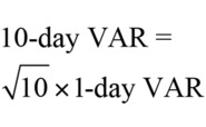
Under current regulations, VAR (when based on either current or stressed data) is calculated using a 10-day horizon. For the calculation of 10-day VAR under existing regulations, the Basel Committee allows the following formula to be used:

This means only one-day changes are considered. The formula is exactly true when daily losses – and gains – have independent normal distributions with a mean of zero and is approximately true in other situations. Under the proposed new rules, the time horizon used for a market variable will be between 10 and 250 days dependent on its liquidity. For example, a time horizon of 10 days will be used for the price of a large-cap stock while a time horizon of 120 days will be used for the credit spread of a non-investment-grade corporate.

Advantages of expected shortfall

As Artzner et al (1999) pointed out some time ago, ES has better theoretical properties than VAR. If two portfolios are combined, the total ES usually decreases - reflecting the benefits of diversification – and certainly never increases. By contrast, the total VAR can – and in practice occasionally does – increase. This is discussed in Hull (2006). To use the terminology of Artzner et al, ES is "coherent" because it has certain fundamental properties they consider such a measure should have. In particular, ES never increases as portfolios are diversified. VAR is not coherent because it does not have this particular property.

There is a more pragmatic reason for preferring ES to VAR in risk management. It is tempting for a trader to follow a trading strategy that is nearly always profitable, but occasionally blows up.⁵ This strategy should be prevented by an ES risk limit, but may be possible when a VAR risk limit is used. Many banks have used ES internally for years, even though VAR is necessary to satisfy regulatory requirements.

Back-testing and accuracy

Expected shortfall has disadvantages as well as advantages, of course. First, it is difficult to back-test. When a one-day 99% VAR model based on the most recent historical data is being back-tested, we can observe the number of exceptions that would have been encountered if the model had been used in the past, and test whether this is significantly different from what is expected. Back-testing a one-day ES model is much more challenging, because we are interested in the average size of the losses when exceptions are observed. A back-testing period of 250 days is usually used by regulators. This can be expected to give about 6 exceptions when a 97.5% confidence limit is used, which is a small sample. However, Acerbi and Szekely (2014) seem to get reasonable results when experimenting with three different tests of ES and standard distributions.

A key point is that back-testing a stressed model, whether VAR or ES, is not possible because we are interested in whether the model performs well for another stressed period, but we do not have another such period to use for testing. The use of varying time horizons in FRTB is an added complication in back-testing.

The Basel Committee has presumably recognised this because the review requires the back-testing of a one-day VAR model calculated in the usual way from recent historical data. We are therefore in the strange position where the risk measure being back-tested is quite different from that used to calculate capital.

Another disadvantage of ES is that estimates of the measure may not be as accurate as estimates of VAR. Yamai and Yoshiba (2002) looked at this. They found that for a certain number of observations and a certain confidence level, the accuracy of VAR and ES is about the same when the loss is normally distributed, but that VAR estimates are more accurate than ES estimates when the losses have fat tails.⁶ This means capital calculated from ES may be less stable than capital calculated from VAR.

Estimating ES

The proposals in the FRTB recommend the use of overlapping time periods for calculations when historical simulation is used. This is markedly different from the square root of time rule mentioned above. One way a historical simulation could be carried out with overlapping time periods is as follows. In the first trial, a shock equal to the change between Day 0 and Day 10 is considered for the price of a large-cap stock, while a shock equal to the change between Day 0 and Day 120 is considered for the credit spread of a non-investment-grade corporate. Other prescribed shocks are considered for other market variables and the loss or gain in the portfolio arising from the shocks is calculated.

The second trial considers a shock equal to the change between Day 1 and Day 11 for the equity price and a shock equal to the change between Day 1 and Day 121 for the credit spread, and so on. The final simulation trial considers a shock equal to the change between Day 249 and Day 259 for the equity price and a shock equal to the change between Day 249 and Day 369 for the credit spread. The ES is then calculated as the average of the losses in the 2.5% tail of the distribution produced by the 250 trials.

Econometricians are likely to take exception to the FRTB recommendation that overlapping time periods be used. Because the changes considered when using overlapping periods are not independent, the effective sample size is much smaller than the actual sample size. As a result, although the estimate is not biased, it is very noisy. In our example, some daily credit spread changes for a non-investment-grade corporate occurring during the 250-day stressed period would be included 120 times in the 250 historical simulations. If that daily spread change was very large and positive, then it is likely that 120 samples out of the total 250 would be large and positive. The reverse would be true for a single large negative spread change.

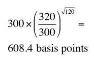
Is there a way in which one-day changes in each market variable are used just once so that the overlapping-time-periods problem is eliminated? Suppose a non-investment-grade credit spread increases from 300 to 320 basis points in a day. What credit spread at the end of 120 days is equivalent to 320 at the end of one day? By this we mean: what percentile of the distribution of the credit spread in 120 days is the same as the percentile observed for the credit spread after one day?

One simple idea is as follows. Assume changes in the logarithm of the credit spread on successive days are independent normal distributions with zero mean and a constant standard deviation. The equivalent credit spread at the end of 120 days is:

This estimate can be criticised in a number of ways. First, assuming the change in the logarithm of the credit spread is zero is not the same as assuming the change in the credit spread itself is zero. To correct for this, we need to know the volatility of the credit spread. Second, the volatility is not constant. If we estimate a Garch (1, 1) model, the estimate can be revised to take account of expected changes in the volatility.⁷ Third, the changes in successive days may exhibit autocorrelation, with positive autocorrelation increasing the estimate, while negative autocorrelation decreases it. This can also be adjusted for.⁸

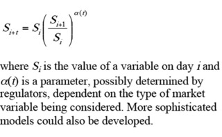
One approach to avoid different banks using different models would be for regulators, based on empirical research, to prescribe how one-day changes should be converted to the required t-day changes for the purposes of the historical simulation. A simple rule could involve setting

An alternative to this is to abandon historical simulation and switch to a model-building approach in conjunction with Monte Carlo simulation. This would involve fitting a model for market variables to stressed market conditions and using it to sample changes in the variables over the prescribed number of days. In the early days of VAR, some banks used a model-building approach and some used historical simulation to calculate the measure. Eventually, historical simulation became regarded as the best approach and is now used by almost all banks. We may well go through a similar process, as banks use different approaches to implement FRTB. Whether historical simulation or model building emerges as the victor remains to be seen.

John Hull and Alan White are professors of finance at the University of Toronto's Joseph L Rotman School of Management. The fourth edition of John Hull's book Risk Management and Financial Institutions will be published by Wiley in early 2015.

Footnotes

¹ See Basel Committee on Banking Supervision (2013).
² See Hull (2015), chapter 17 for a more complete description of the changes proposed in the FRTB.
³ ES is the expected loss conditional on the VAR level of losses being exceeded. ES is also referred to as C-VAR, conditional tail expectation, and expected tail loss.
⁴ Currently market risk capital is calculated as the sum of an amount based on current VAR and an amount based on stressed VAR, the latter being calculated over a similar worst-250-day period.
⁵ A simple example of such a strategy would be the sale of deep-out-of the money options. Strategies that work well except when there are unusual market moves, such as a "flight to quality", can also fall into this category.
⁶ However, the ES in FRTB has a 97.5% rather than a 99% confidence level. The lower confidence level should improve the accuracy of the ES estimate somewhat.
⁷ See Hull (2014), chapter 23.
⁸ See Hull (2015), chapter 12.

References

Acerbi C and B Szekely (2014)
Backtesting Expected Shortfall
Forthcoming article in Risk

Artzner P, F Delbaen, J-M Eber and D Heath (1999)
Coherent Measures of Risk
Mathematical Finance, 9, 203-228

Bank for International Settlements (October 2013)
Consultative Document: Fundamental Review of the Trading Book: A Revised Market Risk Framework

Hull J (2014)
Options, Futures, and Other Derivatives
Ninth edition, Upper Saddle River, NJ, Pearson

Hull J (2015)
Risk Management and Financial Institutions
Fouth edition, Hoboken, Wiley

Hull J (2006)
VAR vs. Expected Shortfall
Risk December

Yamai Y and Yoshiba T (2002)
Comparative Analysis of Expected Shortfall and Value at Risk: Their Estimation Error, Decomposition, and Optimization
Monetary and Economic Studies, January, 87-121

FRTB – a timeline

• Risk management

Banks make new push on FRTB’s P&L test

• 08 Mar 2018

• Regulation

Basel delay does not ensure global FRTB consistency

• 18 Dec 2017

• Regulation

Basel rules risk fragmentation after key compromise

• 07 Dec 2017

• Risk management

ECB tells IMA banks to apply before rules are complete

• 19 Oct 2017

• Risk management

FRTB: industry pushes to use own quotes in risk factor modelling

• 08 Sep 2017

• Basel Committee

EU lawmakers consider extending FRTB deadline

• 24 May 2017