Journal of Investment Strategies
ISSN:
2047-1246 (online)
Editor-in-chief: Ali Hirsa
Tail-risk mitigation with managed volatility strategies
Anna A. Dreyer and Stefan Hubrich
Need to know
- The Sharpe Ratio benefit of managed volatility strategies is period dependent.
- Volatility stabilization consistently removes tail risk from the return distribution.
- The tail risk enhancement is economically meaningful within a utility-based framework.
Abstract
Managed volatility strategies adjust market exposure in inverse relation to a risk estimate, to stabilize realized portfolio volatility through time. Our paper examines strategy performance from an investment practitioner perspective. Using long-term data from the Standard & Poor’s 500, we show that these strategies offer an improvement in risk-adjusted return compared with a buy-and-hold benchmark, on average, but with some variation. Managed volatility strategies achieve robust tail-risk reduction while also enhancing skewness. These return normalization features are inherently linked to the nature of the volatility stabilization mechanism. We illustrate them via utility-based metrics that reward the tail-risk reduction emanating from volatility stabilization. These enhancements are economically meaningful for many time horizons and holding period combinations, and they remain once transaction costs have been included, suggesting a durable and tangible value-add from managed volatility strategies. They also suggest a more appropriate way to measure the performance improvements of tail-risk-mitigating strategies.
Introduction
1 Introduction
Managed volatility strategies adjust market exposure in inverse relation to a risk estimate, with the aim of stabilizing realized portfolio volatility through time. While volatility stabilization is achievable with relative ease, owing to the general predictability of volatility, or volatility clustering, it is not by itself of obvious benefit to investors. Advocates for these strategies typically argue that they also provide higher risk-adjusted returns, most likely due to countercyclicality in the risk/return relationship of the underlying equity market itself. A robust and broadly constructive empirical body of literature has developed on this topic over the last decade, but the time periods and success metrics used vary greatly, leaving investors wanting for a robust set of stylized facts as their guide. Our paper examines managed volatility performance under a range of success metrics that align with how investment practitioners often evaluate investment strategies, including explicit consideration of a time horizon (holding period). We rely on a much longer data set than is typically seen in the volatility management literature. We employ a utility-based approach as a way of capturing the effect of the strategy on higher moments. Our key finding is that, while managed volatility is associated with varying improvements in risk-adjusted return, it produces robust enhancements in tail-risk reduction. We believe this perspective is both novel and important because it refocuses the case for the strategy on its inherent risk management characteristics, rather than being a targeted focus on its risk-adjusted performance enhancement, as tail-risk reduction is a direct consequence of the volatility stabilization mechanism.
Perchet et al (2014a) provide a useful conceptual framework by examining, both theoretically and through simulation, a wide range of conditions under which Sharpe ratio enhancement from managed volatility can arise. When applying their approach to Standard & Poor’s 500 (S&P 500) data (1990–2012), they find a meaningful Sharpe ratio improvement. Perchet et al (2014b) apply the same approach to factor returns. Hallerbach (2012) focuses more on the theoretical argument for the superiority of managed volatility portfolios, but he also demonstrates a Sharpe ratio improvement for European equity markets over the 2003–11 period. Moreira and Muir (2017) put their emphasis on the conditional Sharpe ratio of the underlying asset as the main channel for Sharpe ratio improvements in managed volatility portfolios.11 1 If forward volatility is predictable but the forward return is not related to the volatility forecast, then volatility forecasts also predict time-varying Sharpe ratios that are higher when volatility is predicted to be low. The assumption that forward returns are entirely unrelated to predicted volatility also leads Moreira and Muir (2017) to focus on “variance-managed” portfolios, which allocate to equities in inverse relation to expected variance rather than expected standard deviation. Our paper makes the baseline assumption that Sharpe ratios are invariant to predicted risk, which implies allocating inversely to standard deviation rather than variance. Using a wide range of underlying assets and assuming a Sharpe ratio maximizing mean–variance investor, they find Sharpe ratio improvements from managed volatility in a wide range of cases.
Fleming et al (2001) use a quadratic utility approach and find meaningful improvements from managed volatility portfolios, albeit over a somewhat narrow time period (1983–97). In Fleming et al (2003), the same group of authors demonstrates the benefit of using intraday “realized” volatility for the volatility forecast. Another highly relevant paper is Hocquard et al (2013), which focuses on tail-risk mitigation from managed volatility strategies, employing a sophisticated payoff transformation procedure to explicitly target a certain realized return distribution. Looking at a global equity portfolio for the 1990–2011 period, the authors find meaningful tail-risk reduction in addition to a substantial Sharpe ratio improvement. Using a utility-based approach, they are able to holistically score all aspects of the return. Similarly, Moreira and Muir (2016) calibrate outright structural models to empirical data in order to include a wider range of utility preferences. They find large utility improvements from managed volatility portfolios.22 2 We also note that there is a related and older literature dealing with the conditional Sharpe ratio of the underlying equity markets. We do not review this literature in detail, referring the reader instead to some of the more recent papers: Lettau and Ludvigson (2010), Brandt and Kang (2004), Lundblad (2007) and Tang and Whitelaw (2011), and the references therein. In the existing literature, the paper by Dopfel and Ramkumar (2013) is most similar to ours. Like this paper, they use a relatively long historical sample (starting in 1950) and employ utility-based analysis. Focusing on quarterly holding periods, they find a small Sharpe ratio improvement and a more meaningful utility improvement from managed volatility strategies. However, they do not explicitly recognize the link between the greater utility improvement and the impact of the strategy on the higher moments of return (tail-risk hedging). To draw out that link is the main point of our paper. We also expand on their work by considering results across a range of possible investor holding periods, and by using higher-frequency data (daily rather than quarterly), which helps our findings to align better with how investors likely employ the strategy in practice. Finally, Dreyer et al (2016) make a relevant contribution to the literature by illustrating how managed volatility strategies can be combined with other strategies for portfolio enhancement.
2 Why might managed volatility be worth having?
Managed volatility (MV) strategies rely on the ability to forecast near-term risk. As a simple illustration, consider that across our sample covering US equity market data since 1926 (see our first appendix (available online) for data sources and calculation details), the return correlation between adjacent sixty-trading-day periods is essentially zero. In contrast, the correlation rises to 0.55 for risk as measured by standard deviation. Past returns do not predict future returns, but past volatility certainly predicts future volatility.
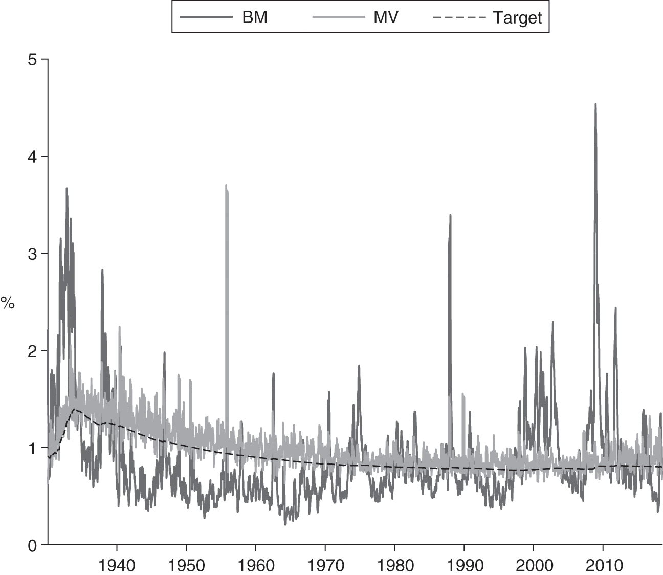
The immediate use case for this ability to forecast risk is to stabilize realized portfolio volatility. This can be accomplished by frequently recalibrating equity market exposure such that the expected portfolio volatility under the forecast aims at a constant target. Figure 1 illustrates this concept. We show the rolling realized sixty-day volatility for two portfolios: the raw equity market (the static benchmark) and a stylized MV strategy.33 3 The MV strategy dynamically alters the daily equity market exposure according to the ratio of realized past long-term equity volatility and the trailing twenty-day realized volatility. The former represents the volatility target and the latter, the forecast. Figure 1 clearly shows the volatility stabilization attribute of the MV strategy, as its realized volatility consistently hugs the target volatility within a much tighter range than the benchmark. This observation holds even during turbulent market episodes such as the mid-1970s, the 1987 crash, the tech bubble/crash of the early 2000s and the global financial crisis (GFC) of 2008–9.
There are several investment applications where this volatility stabilizing feature is valuable. The primary example is the variable annuity industry, where many policies are sold with guarantees pertaining to a certain withdrawal stream from the underlying assets. That liability resembles a complex equity index option portfolio, and, by applying MV strategies to the underlying assets, insurers can stabilize and even reduce the hedging costs associated with their variable annuity book.
Second, stabilizing volatility can also enhance the suitability of portfolios that advisors manage for their clients. Client portfolios are often picked from a range of models with different long-term risk characteristics, based on questionnaires and client preferences expressed elsewhere. A traditional model, like the line labeled “BM” in Figure 1, likely exhibits a fluctuating volatility profile that often differs from the long-term “bucket” in which the client has been placed. MV strategies could be deemed more suitable, as their risk characteristics are more stable through time.
Third, individual investors often overreact to fluctuations in volatility by selling out of risky strategies at inopportune times. See Kinnel (2015) for a study along those lines, which compares investment returns to investor returns, with the latter also capturing the timing of buy and sell decisions. The author demonstrates that this gap widens with the volatility of the underlying investment. Hence, an MV strategy that attenuates the benchmark fluctuations shown in Figure 1 may reduce adverse trading behavior and close this gap.
The dynamic allocation process inherent in MV can seem antithetical to the value-conscious, somewhat contrarian nature of many professional investors. Equities tend to be cheap when volatility is high. Interestingly, Moreira and Muir (2017) illustrate that market valuation signals and MV strategies are complementary. Their key insight is that valuation is best at forecasting returns for very long time horizons, while MV strategies tend to react dynamically to shorter-term trends in volatility. As long as the gains from attractive valuations are harvested in the long term rather than immediately following an attractive valuation observation, MV does not lose much expected return by lowering exposure immediately after a sell-off. It is entirely possible that most of the long-term future gains from a low valuation starting point are harvested during normal or even low-volatility periods, when MV features healthy equity exposure.

We also need to recognize that MV strategies can and will routinely employ leverage, here defined as equity exposure in excess of 100% during low-volatility episodes. The strategy depicted in Figure 1 employs leverage on 64% of days.44 4 The illustrated strategy is unconstrained and rebalanced daily. The mean and median daily equity exposures are 134% and 122%, respectively.55 5 Daily equity exposure at the 10th, 25th, 75th and 90th percentiles is 57%, 83%, 171% and 224%, respectively.
The use of leverage during low-volatility periods allows MV to garner excess returns over the benchmark during these periods if the underlying market returns are positive. As such, outperformance of MV strategies in calm periods, such as 2017, is often overlooked. It is the main feature that can compensate for opportunities lost by de-risking in crisis periods. MV would employ leverage whenever the short-term volatility forecast for the underlying market falls below the long-term target. In Figure 1, these periods are largely consistent with the benchmark short-term volatility falling below the target. The larger the deviation, the larger the degree of leverage. However, in high-volatility periods, MV also significantly reduces exposure below 100%.
Further, return as the key measure of success becomes meaningless for strategies that can employ leverage. As long as the underlying market returns are positive on average, additional leverage can be applied to achieve the desired return target. Therefore, what matters is risk-adjusted return: how much return does the portfolio garner per unit of risk? We will focus on the Sharpe ratio (SR), defined as the average excess return divided by standard deviation, as the most commonly used metric for risk-adjusted return. Our question then becomes the following: why/when would we expect MV to have a higher SR than the benchmark? The literature provides us with several relevant considerations here (see Perchet et al (2014a) for a detailed study on this topic). The primary driver is the conditional SR of the underlying equity market itself. There is a large body of existing literature suggesting that, broadly speaking, realized equity market SR is lower when risk is high. This is referred to as market level SRs being countercyclical. It would make MV an excellent market timing device, featuring more exposure when market level risk/reward is attractive (volatility is low), and vice versa. In fact, the MV strategy contemplated here, which scales exposure inversely to volatility rather than variance, would be suboptimal. As shown in Moreira and Muir (2016), the optimal strategy in the extreme case of expected returns that are invariant to predicted volatility would be a “variance-managed” portfolio that allocates to the equity market inversely to predicted variance.
We focus our study on MV relative to standard deviation because it is defensible under much weaker conditions: if the equity market SR is at least constant, MV should not fall below the benchmark with regard to the long-term SR (Kolanovic and Wei 2013). Outright countercyclicality is unnecessary. As practitioners, we also note that MV strategies – as we define them – constitute an actual investment category in the market place. Further, the results of our paper themselves support our approach. While we generally find improvements in the SR historically, the degree of this improvement is period dependent. We also demonstrate that volatility-stabilized strategies have distinct tail-risk hedging benefits that can and do accrue in the absence of time-varying market level SRs.66 6 A second reason to expect a higher SR from MV lies in its longitudinal diversification benefits. By targeting constant risk through time, each period allocates equally to the time series risk of the MV return stream. In theory, this should provide better risk-adjusted returns, much like the effect of cross-sectional diversification. In the extreme case of uncorrelated assets, the SR maximizing point-in-time portfolio will allocate equal risk to each asset. Perchet et al (2014a) investigate this angle but conclude that, in practice, this benefit is not economically meaningful.
Last, if an MV long-term SR does not fall below that of the underlying equity market, as Kolanovic and Wei (2013) suggest, and leverage can be applied, the compound returns of MV should approximately scale with the target volatility.77 7 The impact of MV on risk-adjusted returns should be relatively independent of the volatility target if cash is used as the de-risking asset to avoid asset allocation effects. In this paper, we have selected a target level of volatility consistent with the underlying equity market. However, other levels of fixed or varying target volatility could have been selected. This is commonly done in practitioner portfolios. In these cases, different degrees of leverage could be applied by reducing the allocation to the underlying equity market, thus reducing the compound return and volatility while retaining the risk-adjusted return. This paper does not use fixed target volatility to avoid lookahead bias in selecting the fixed target.
3 Traditional risk-adjusted performance evaluation
We focus our analysis on US data, which provides us with a very long-term sample of daily returns, starting in 1926. One of our key concerns is stability of findings through time. Several studies have established MV attributes for a wide range of assets, but our concern is that the emphasis on breadth restricts them to a sample length of no more than two to three decades, a sample heavily influenced by the GFC. We believe that our US-only, but very long-term, study provides an important cross-check to those findings.88 8 In addition, global equity markets are strongly correlated, especially during periods of turbulence. This correlation has increased as global markets have become increasingly interconnected. We believe that looking at a longer longitudinal sample, as opposed to one with broader regional representation, offers a more powerful robustness test.
We focus on two forms of robustness in the time dimension: across sample periods, and across holding periods within each sample period. The holding period is the frequency at which the investor evaluates performance. In other words, it is the time window over which individual return observations are cumulated. Here, holding period refers only to the window length over which daily returns are aggregated, not the rebalancing frequency.99 9 See, for example, Perchet et al (2014a) for an MV study employing lower-frequency rebalancing periods. Our data is daily, and we permit daily trading. We view the problem through the lens of an investment manager offering an MV product. That product may have a diverse investor base with a variety of holding periods of interest. Thus, our focus is on an unconstrained, daily traded MV strategy that has the potential to maximize benefits from volatility management. In our experience as practitioners, these strategies are actually managed in this manner. They can be rebalanced daily, as warranted by changes in the volatility signal used, and they can include large daily trades in liquid futures to adjust the risk profile.1010 10 We do acknowledge that investment practitioners will likely put some guardrails around daily trading behavior, however, and our second appendix (available online) re-evaluates key results under such constraints; they are unaffected by these considerations.
Table 1 presents our findings concerning traditional and risk-adjusted performance.1111 11 The MV series shown in Table 1 are constructed using a twenty-day trailing realized volatility estimate as the forecast. Metrics are shown based on returns in excess of cash and are not annualized. See the online appendix for further information. For a baseline MV strategy relying on trailing twenty-day realized volatility as its forecast, the longest sample (starting in 1929) features meaningful SR improvements to the order of 20–30% for holding periods up to a quarter. The deterioration of the improvement as the holding period lengthens is noteworthy, however. Our analysis confirms the notion that truly long-term investors, with holding periods beyond one year, should not expect much of an enhancement from MV strategies. In fact, we see a degree of SR underperformance from MV strategies at these horizons. It seems that for a long enough horizon, the long-term growth potential and mean-reversion tendencies of equity markets are the more important principle.1212 12 See Moreira and Muir et al (2017) for a confirmatory and quite nuanced discussion of the role time horizons play in the comparison between MV strategies and valuation centric strategies. We also compute the (nonannualized) alpha for each holding period.1313 13 Alpha regression allows for variable beta to the benchmark. While the alpha is positive up to a three-year holding period, the marginal improvement in the alpha begins to degrade for holding periods beyond three months. Alphas are significant for up to one year when using data starting in 1926, but they are only significant for holding periods up to one day and one month, respectively, when using data starting in 1960 and 1990.
The degree of the SR enhancement from MV varies based on the time period of interest. We first show this in Table 1 by also providing results for subperiods starting in 1960 and 1990.1414 14 For each holding period, we construct all nonoverlapping histories possible based on daily returns, aggregate returns to the holding period, calculate the statistic within each history and then average the statistics across histories. These statistics are not annualized. This approach is used for the results shown in all tables. All returns are in excess of cash. MV is constructed using trailing twenty-day realized volatility as the volatility forecast. Bootstrap 90% confidence intervals (5th and 95th bootstrap percentiles) on differences in SRs shown between MV and the benchmark are displayed. See the first appendix (available online) for details on data and analysis. The smallest improvement is seen for the period starting in 1960. For the period starting in 1990, we again see improvements, but these are not quite as material as when we start in 1929. Confidence intervals contain positive differences only for the 1929 period for horizons up to sixty days. It is worth emphasizing that this last sample period, and the various subperiods therein, is the most frequently used in the existing literature.
| 20 days | 60 days | 240 days | 720 days | 2400 days | ||||||||
|---|---|---|---|---|---|---|---|---|---|---|---|---|
| 1 day | (1 month) | (3 months) | (1 year) | (3 years) | (10 years) | |||||||
| BM | MV | BM | MV | BM | MV | BM | MV | BM | MV | BM | MV | |
| 1929–2018 | ||||||||||||
| Annualized | 5.99% | 8.10% | ||||||||||
| geometric | ||||||||||||
| return | ||||||||||||
| Average | 0.03% | 0.04% | 0.59% | 0.78% | 1.80% | 2.39% | 7.43% | 10.32% | 23.99% | 35.15% | 98.75% | 171.83% |
| return | ||||||||||||
| Risk (SD) | 1.06% | 1.06% | 5.06% | 5.56% | 9.32% | 10.27% | 19.07% | 25.49% | 33.38% | 55.58% | 89.45% | 189.68% |
| Sharpe ratio | 2.71% | 3.45% | 11.65% | 13.97% | 19.36% | 23.23% | 39.00% | 40.57% | 72.49% | 63.87% | 111.76% | 92.87% |
| Difference in | 0.74% | 2.32% | 3.87% | 1.57% | 8.62% | 18.89% | ||||||
| Sharpe ratio | ||||||||||||
| 90% CI of | [0.1%, 1.4%] | [0.3%, 4.4%] | [0.4%, 7.1%] | [5.0%, 7.0%] | [21.1%, 2.2%] | [75.7%, 2.7%] | ||||||
| Sharpe ratio | ||||||||||||
| difference | ||||||||||||
| Alpha (bps) | 1.27 | 22.31 | 70.45 | 185.98 | 158.40 | 2023.67 | ||||||
| 90% CI of | [0.6, 1.9] | [11.1, 32.2] | [32.8, 104.4] | [41.7, 308.3] | [329.6, 531.5] | [5780.5, 634.9] | ||||||
| Alpha (bps) | ||||||||||||
| 1960–2018 | ||||||||||||
| Annualized | 5.30% | 6.31% | ||||||||||
| geometric | ||||||||||||
| return | ||||||||||||
| Average | 0.03% | 0.03% | 0.52% | 0.63% | 1.57% | 1.92% | 6.46% | 7.95% | 18.77% | 22.88% | 63.35% | 79.83% |
| return | ||||||||||||
| Risk (SD) | 0.97% | 0.97% | 4.40% | 5.04% | 7.73% | 9.00% | 16.10% | 19.21% | 27.93% | 34.93% | 64.50% | 89.06% |
| Sharpe ratio | 2.60% | 2.99% | 11.71% | 12.43% | 20.31% | 21.33% | 40.24% | 41.40% | 67.42% | 65.75% | 106.21% | 91.08% |
| Difference in | 0.39% | 0.72% | 1.01% | 1.16% | 1.67% | 15.13% | ||||||
| Sharpe ratio | ||||||||||||
| 90% CI of | [0.3%, 1.1%] | [1.7%, 3.2%] | [3.8%, 5.3%] | [8.2%, 9.1%] | [17.4%, 12.0%] | [231.8%, 14.7%] | ||||||
| Sharpe ratio | ||||||||||||
| difference | ||||||||||||
| Alpha (bps) | 0.75 | 10.88 | 30.97 | 107.27 | 293.64 | 582.41 | ||||||
| 90% CI of | [0.1, 1.4] | [1.6, 22.5] | [7.2, 67.1] | [53.6, 252.1] | [164.7, 771.4] | [7254.6, 971.9] | ||||||
| Alpha (bps) | ||||||||||||
| 1990–2018 | ||||||||||||
| Annualized | 7.02% | 8.85% | ||||||||||
| geometric | ||||||||||||
| return | ||||||||||||
| Average | 0.03% | 0.04% | 0.65% | 0.81% | 1.97% | 2.44% | 8.37% | 10.36% | 26.09% | 32.97% | 74.32% | 99.62% |
| return | ||||||||||||
| Risk (SD) | 1.10% | 1.10% | 4.39% | 4.75% | 7.48% | 8.33% | 16.03% | 19.20% | 33.43% | 42.43% | ||
| Sharpe ratio | 2.99% | 3.61% | 14.88% | 17.03% | 26.35% | 29.39% | 52.55% | 54.20% | 79.47% | 78.90% | ||
| Difference in | 0.61% | 2.16% | 3.04% | 1.65% | 0.57% | |||||||
| Sharpe ratio | ||||||||||||
| 90% CI of | [0.4%, 1.7%] | [1.6%, 5.8%] | [4.4%, 9.9%] | [16.7%, 10.6%] | [21.4%, 32.2%] | |||||||
| Sharpe ratio | ||||||||||||
| difference | ||||||||||||
| Alpha (bps) | 1.16 | 19.24 | 53.68 | 161.20 | 404.73 | |||||||
| 90% CI of | [0.0, 2.2] | [3.0, 36.4] | [6.7, 107.9] | [116.1, 311.7] | [248.2, 1302.9] | |||||||
| Alpha (bps) | ||||||||||||

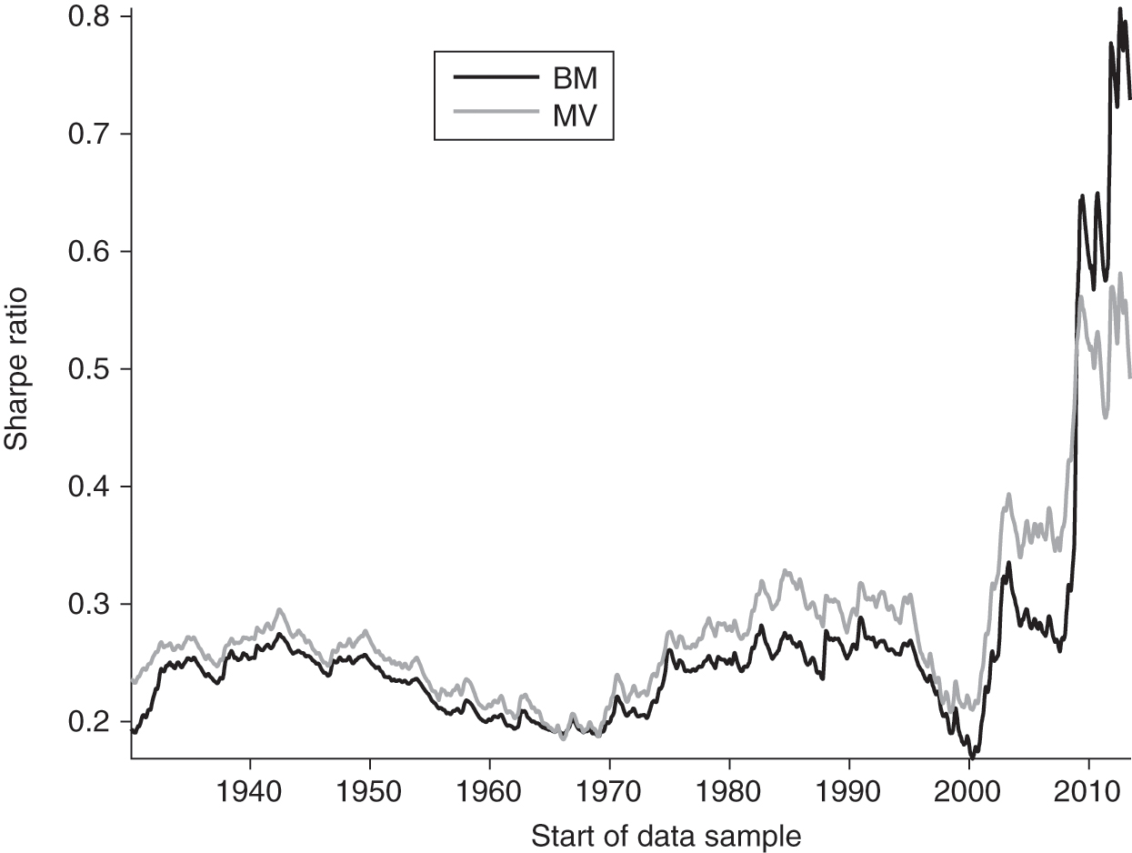
Another way to evaluate robustness is shown in Figure 2. This displays the benchmark and MV SR that arises in the sample, beginning with the time indicated on the horizontal axis and ending in June 2018 (the end of our sample). This visual aid illustrates the impact of the starting period on the risk-adjusted performance of MV compared with the benchmark. We start the chart on the right in June 2013, assuming that any backtest would show at least five years of data. Starting the backtest in 2013, the benchmark outperforms MV with a higher SR. MV only begins to have a better SR when the GFC is included, starting in 2007. From then on, the two remain close until the Great Depression, which finally gives MV its edge for the full sample. It is fair to say that this is not a robust picture for those looking for a reliable SR improvement from MV. Investors pursuing pure MV strategies for SR enhancement should consider the potential for regret risk, even with a long-term commitment to the strategy.
| 20 days | 60 days | 240 days | 720 days | 2400 days | ||
|---|---|---|---|---|---|---|
| 1 day | (1 month) | (3 months) | (1 year) | (3 years) | (10 years) | |
| Benchmark | 2.71 | 11.65 | 19.36 | 39.00 | 72.49 | 111.76 |
| MV (10-day) | 3.49 | 14.04 | 23.56 | 41.25 | 64.16 | 82.06 |
| MV (20-day) | 3.45 | 13.97 | 23.23 | 40.57 | 63.87 | 92.87 |
| MV (30-day) | 3.31 | 13.37 | 22.16 | 38.55 | 62.84 | 88.29 |
| MV (60-day) | 3.30 | 13.40 | 22.30 | 38.01 | 60.25 | 81.67 |
Pure MV strategies are characterized by material turnover and trading activity due to their dynamic adjustment of exposures, permitting equity exposure that can be dramatically different from the benchmark for periods of time. Not all investors have an appetite for such high turnover or tracking error to the static benchmark. Varying the forecast horizon via its trailing window length is one convenient way of sizing the degree to which MV is added to the portfolio, as volatility forecasts based on longer windows inherently lead to more stable exposures. Further, a naive notion of symmetry might suggest using longer trailing windows, and thus slower moving forecasts, if the MV strategy is evaluated over a longer holding period, and vice versa. To investigate this further, Table 2 shows how the key results for the longer sample period starting in 1929 are affected when using trailing windows longer or shorter than the twenty days employed so far for forecasting volatility.
Perhaps surprisingly, short windows with more responsive forecasts are superior even for longer holding periods. Of course, even though we may evaluate over a longer holding period, the strategy will still adjust exposure daily. It thus makes sense that the dynamics of the forecast should be governed by the trading frequency and not by the evaluation period. One implication is that if turnover or tracking error present a material concern, it may be more effective to manage them directly via explicit constraints on portfolio construction, rather than by weakening the forecasting power of the algorithm. The role of the volatility forecast is to provide the best projection of volatility over the next trading period.
4 The link between managed volatility and tail risk
We now turn to the impact of MV on the higher moments of the return distribution. These outcomes are not captured by the traditional metrics of risk-adjusted returns based on the first two moments: average return and volatility. In Section 5, we will see that evaluating tail-risk properties presents a bridge to a more holistic perspective on MV investor benefits.
Table 3 summarizes the key tail-risk metrics of the same MV strategies and sample/holding periods underlying the analysis in Table 1. We start by showing the third and fourth standardized moments of the return distribution: skewness and kurtosis. Skewness measures the asymmetry of the return distribution, and kurtosis measures the fatness of the tails. Investors naturally prefer high positive skewness and low kurtosis. Portfolio-level kurtosis indicates that MV consistently thins the tails at twenty- and sixty-day holding periods. At these holding periods, the benchmark features meaningful excess kurtosis, while MV essentially produces normal tails with kurtosis close to . As holding periods increase, return distributions become more normal.1515 15 This is the natural effect of the law of large numbers when aggregating returns over time, producing increasingly normally distributed sums even if the individual returns are not normal. However, the normalization can be seen at shorter holding periods for MV than for the benchmark. Bootstrap confidence intervals include the number 3, starting with a sixty-day holding period for MV, but not until one year for the benchmark.1616 16 A kurtosis value of 3 is consistent with a normal return distribution. This effect on shorter-term kurtosis is present in most periods of our sample (see the second appendix, available online). With few exceptions, MV skew confidence intervals tend to be narrower and closer to, or more likely to include, zero than the benchmark, supporting the tendency of MV to normalize return distributions.
Table 3 also shows measures of absolute tail risk in the form of 5% and 1% conditional value-at-risk (CVaR). These represent the average of the bottom 5% and 1%, respectively, of relevant holding period returns. MV features notable, but time-period-dependent, improvements, roughly similar to the SR pattern in Table 1. We must keep in mind, however, that absolute tail risk is also a function of the level of volatility itself. As can be seen clearly in Table 1, MV strategies feature greater absolute volatility as well as greater average returns at longer holding periods.1717 17 This is perhaps surprising since MV is calibrated to match the volatility of the benchmark, albeit at daily frequency. We hypothesize that this is due to the asymmetric impact of volatility estimation error on positioning. Since MV sets equity exposure inversely to volatility forecast, an underestimation of true volatility adds more to portfolio risk than an overestimation by the same amount would detract. From an investor perspective, the volatility gap between benchmark and MV should not be too much of a concern per se, as one can directionally calibrate the MV strategy to a lower ex-ante volatility profile in order to compensate for the impact of forecast error on realized volatility. The generally lower CVaR of MV strategies is thus remarkable, as it occurs against a backdrop of having higher volatilities. If higher volatilities are also associated with higher returns, these absolute tail-risk properties could be more attractive than it may seem at first blush. We home in on this aspect by also showing a metric that divides the annualized return by the size of the CVaR. This metric neutralizes the impact of higher baseline volatility if that volatility is accompanied by higher returns, as would be the case if the SR remains constant. For these metrics, Table 3 paints a picture of robust superiority of MV strategies, regardless of time horizon or sample period. The positive impact for longer holding periods is particularly noteworthy.1818 18 Upon examining these cases, it seems that skewness improvements can play a role here, even when kurtosis is not reduced compared with the benchmark. Clearly, for the same level of kurtosis, a larger skew can improve the CVaR, as more of that tail now resides in the positive return extreme which the CVaR does not capture.
| 20 days | 60 days | 240 days | 720 days | 2400 days | ||||||||
| 1 day | (1 month) | (3 months) | (1 year) | (3 years) | (10 years) | |||||||
| BM | MV | BM | MV | BM | MV | BM | MV | BM | MV | BM | MV | |
| 1929–2018 | ||||||||||||
| Skewness | 0.02 | 1.32 | 0.14 | 0.21 | 0.87 | 0.28 | 0.14 | 1.15 | 0.12 | 1.42 | 0.58 | 0.94 |
| 90% CI of | [0.5,0.4] | [2.5,0.5] | [0.6,0.7] | [0.3,0.1] | [0.3,1.6] | [0.1,0.4] | [0.5,0.2] | [0.5,1.5] | [0.2,0.5] | [0.5,1.7] | [0.4,1.0] | [0.1,1.4] |
| skewness | ||||||||||||
| Kurtosis | 18.25 | 26.71 | 10.88 | 3.99 | 13.16 | 3.43 | 3.94 | 6.14 | 3.02 | 5.70 | 2.72 | 2.85 |
| 90% CI of | [13.0,24.1] | [7.6,57.5] | [6.8,13.6] | [3.6,4.4] | [5.7,15.9] | [3.0,3.8] | [3.2,4.4] | [3.4,7.5] | [2.4,3.5] | [2.9,7.0] | [1.5,3.4] | [1.4,4.0] |
| kurtosis | ||||||||||||
| 5% CVaR | 2.54% | 2.54% | 11.70% | 11.73% | 19.52% | 17.60% | 34.81% | 31.23% | 37.90% | 37.13% | 19.13% | 21.23% |
| 90% CI of | [0.1%,0.4%] | [0.2%,3.4%] | [1.3%,7.3%] | [1.1%,11.7%] | [4.9%,5.8%] | [11.3%,12.6%] | ||||||
| 5% CVaR | ||||||||||||
| difference | ||||||||||||
| 1% CVaR | 4.36% | 4.20% | 18.32% | 16.63% | 27.78% | 23.07% | 48.83% | 38.38% | 47.54% | 43.68% | 19.13% | 21.23% |
| 90% CI of | [0.1%,0.1%] | [0.8%,0.8%] | [0.0%,3.9%] | [1.0%,7.1%] | [5.5%,4.9%] | [7.2%,12.6%] | ||||||
| 1% CVaR | ||||||||||||
| difference | ||||||||||||
| Mean/ | 1.13% | 1.44% | 5.03% | 6.63% | 9.26% | 13.57% | 21.48% | 33.18% | 69.99% | 97.72% | 262.77% | 836.00% |
| (5% CVaR) | ||||||||||||
| Mean/ | 0.66% | 0.87% | 3.22% | 4.68% | 6.55% | 10.40% | 15.58% | 27.18% | 58.06% | 84.10% | 262.77% | 836.00% |
| (1% CVaR) | ||||||||||||
| 1960–2018 | ||||||||||||
| Skewness | 0.53 | 0.56 | 0.65 | 0.21 | 0.47 | 0.11 | 0.43 | 0.03 | 0.01 | 0.41 | 0.13 | 0.29 |
| 90% CI of | [1.2,0.1] | [0.8,0.4] | [0.9,0.3] | [0.3,0.1] | [0.7,0.1] | [0.1,0.3] | [0.7,0.1] | [0.2,0.2] | [0.3,0.4] | [0.0,0.7] | [0.6,0.6] | [0.4,0.7] |
| skewness | ||||||||||||
| Kurtosis | 18.87 | 6.69 | 6.27 | 3.32 | 4.89 | 3.18 | 3.12 | 2.75 | 2.76 | 3.03 | 2.25 | 1.99 |
| 90% CI of | [10.7,30.4] | [5.1,8.9] | [4.8,7.5] | [3.2,3.5] | [4.0,5.5] | [2.9,3.4] | [2.5,3.7] | [2.4,3.1] | [2.2,3.5] | [2.3,3.5] | [1.2,2.8] | [1.2,2.7] |
| kurtosis | ||||||||||||
| 5% CVaR | 2.28% | 2.25% | 10.38% | 10.64% | 16.92% | 16.00% | 28.56% | 27.94% | 33.70% | 36.69% | 17.11% | 22.69% |
| 90% CI of | [0.1%,0.7%] | [0.2%,4.2%] | [0.5%,7.8%] | [7.5%,7.0%] | [7.3%,3.6%] | [15.0%,9.2%] | ||||||
| 5% CVaR | ||||||||||||
| difference | ||||||||||||
| 1% CVaR | 3.85% | 3.45% | 16.00% | 14.07% | 25.08% | 21.11% | 34.55% | 33.18% | 33.70% | 36.69% | 17.11% | 22.69% |
| 90% CI of | [0.0%,0.1%] | [1.1%,0.6%] | [1.0%,3.0%] | [5.6%,7.2%] | [7.3%,3.6%] | [13.5%,9.2%] | ||||||
| 1% CVaR | ||||||||||||
| difference | ||||||||||||
| Mean/ | 0.01% | 0.01% | 0.05% | 0.06% | 0.09% | 0.12% | 0.23% | 0.29% | 0.58% | 0.63% | 1.85% | 3.72% |
| (5% CVaR) | ||||||||||||
| Mean/ | 0.01% | 0.01% | 0.03% | 0.04% | 0.06% | 0.09% | 0.20% | 0.24% | 0.58% | 0.63% | 1.85% | 3.72% |
| (1% CVaR) | ||||||||||||
| 20 days | 60 days | 240 days | 720 days | |||||||
| 1 day | (1 month) | (3 months) | (1 year) | (3 years) | ||||||
| BM | MV | BM | MV | BM | MV | BM | MV | BM | MV | |
| 1990–2018 | ||||||||||
| Skewness | 0.15 | 0.55 | 0.67 | 0.16 | 0.67 | 0.07 | 0.74 | 0.17 | 0.43 | 0.03 |
| 90% CI of | [0.5,0.3] | [0.7,0.4] | [1.0,0.2] | [0.3,0.0] | [1.1,0.1] | [0.1,0.2] | [1.0,0.3] | [0.4,0.6] | [0.9,0.3] | [0.7,0.7] |
| skewness | ||||||||||
| Kurtosis | 11.33 | 5.99 | 6.47 | 3.09 | 5.59 | 2.69 | 3.67 | 3.01 | 2.30 | 2.48 |
| 90% CI of | [8.9,13.7] | [5.1,7.0] | [5.0,7.6] | [2.8,3.3] | [3.7,6.8] | [2.4,2.9] | [2.4,4.7] | [2.2,3.9] | [1.6,3.0] | [1.6,3.3] |
| kurtosis | ||||||||||
| 5% CVaR | 2.63% | 2.58% | 10.42% | 9.33% | 16.83% | 13.72% | 28.08% | 23.51% | 29.87% | 32.85% |
| 90% CI of | [0.1%,0.7%] | [1.1%,6.7%] | [0.2%,12.8%] | [2.3%,12.2%] | [7.5%,11.0%] | |||||
| 5% CVaR | ||||||||||
| difference | ||||||||||
| 1% CVaR | 4.36% | 4.02% | 15.91% | 12.02% | 23.25% | 16.20% | 33.07% | 25.56% | 29.87% | 32.85% |
| 90% CI of | [0.1%,0.2%] | [0.0%,2.3%] | [0.2%,7.8%] | [2.5%,10.3%] | [7.5%,11.0%] | |||||
| 1% CVaR | ||||||||||
| difference | ||||||||||
| Mean/ | 0.01% | 0.02% | 0.06% | 0.09% | 0.12% | 0.18% | 0.31% | 0.44% | 0.94% | 1.17% |
| (5% CVaR) | ||||||||||
| Mean/ | 0.01% | 0.01% | 0.04% | 0.07% | 0.09% | 0.15% | 0.27% | 0.41% | 0.94% | 1.17% |
| (1% CVaR) | ||||||||||
What is the intuition for the robust tail-risk reduction emanating from MV strategies? We can think of the long-term volatility process as a mixture of distributions, with different distributions being in place at different times.1919 19 See Press (1967), Praetz (1972) and Clark (1973) for early work on this mixture of distribution hypothesis. According to this model, the long-term return patterns exhibiting excess kurtosis and time-changing volatility can result from this mixture of short-term distributions, each with their own inherent volatility. The most extreme observations are generated when conditional volatility is high, and they appear abnormally large relative to the overall volatility of the sample because low- or mid-level-volatility episodes dominate the sample. At the same time, these events are not abnormal when viewed against the conditional distribution that produced them at the time. Fat tails (fourth moment) are merely a byproduct of conditionally elevated volatility (second moment). Due to the short-term persistence of these different volatility regimes, the conditional level of volatility is forecastable. By adjusting exposure inversely to the conditional expectation of volatility, the MV strategy effectively normalizes the overall return distribution, since essentially all portfolio returns are now drawn from roughly the same distribution. In essence, the same phenomenon that causes fat tails, volatility clustering, is also the key feature by which we can predict volatility and use MV to remove fat tails from the return stream. This inherent linkage explains the robustness of the kurtosis improvement. The pattern of volatility regularization shown in Figure 1, which many investors seem to find intuitively preferable, is directly tied to the normalization of the distribution. These characteristics are two sides of the same coin and should be viewed as one and the same benefit. MV will not produce one without the other.
Last, because negative skewness and excess kurtosis reduce compound returns, strategies like MV that normalize the return distributions should increase the compound return. However, leverage is necessary to achieve return normalization without degrading the long-term risk-adjusted return. Reducing the underlying exposure during periods of high volatility normalizes the left tail, while increasing leverage in low-volatility environments provides sufficient excess returns to compensate for reducing risk (and return) in high-volatility episodes.
5 Utility perspective
| 20 days | 60 days | 240 days | 720 days | 2400 days | ||||||||
| 1 day | (1 month) | (3 months) | (1 year) | (3 years) | (10 years) | |||||||
| BM | MV | BM | MV | BM | MV | BM | MV | BM | MV | BM | MV | |
| 1929–2018 | ||||||||||||
| CEV | 4.50% | 6.54% | 4.25% | 6.00% | 4.09% | 5.85% | 3.78% | 5.35% | 4.48% | 5.71% | 5.23% | 6.37% |
| Difference in CEV | 2.05% | 1.75% | 1.76% | 1.57% | 1.23% | 1.15% | ||||||
| 90% CI of CEV | [0.1%,3.8%] | [0.2%,3.2%] | [0.2%,3.4%] | [0.1%,3.1%] | [0.1%,2.6%] | [0.2%,2.8%] | ||||||
| difference | ||||||||||||
| CEV | 2.33% | 3.73% | 2.08% | 2.94% | 1.96% | 2.79% | 1.75% | 2.38% | 2.44% | 2.74% | 3.35% | 3.46% |
| Difference in CEV | 1.40% | 0.85% | 0.83% | 0.64% | 0.29% | 0.11% | ||||||
| 90% CI of CEV | [0.0%,3.7%] | [0.5%,2.7%] | [0.5%,2.8%] | [0.4%,4.0%] | [0.9%,3.0%] | [0.4%,1.7%] | ||||||
| difference | ||||||||||||
| CEV | 1.54% | 2.47% | 1.37% | 1.91% | 1.29% | 1.80% | 1.14% | 1.52% | 1.67% | 1.77% | 2.38% | 2.31% |
| Difference in CEV | 0.93% | 0.54% | 0.51% | 0.39% | 0.10% | 0.07% | ||||||
| 90% CI of CEV | [0.6%,3.7%] | [1.4%,2.2%] | [1.1%,3.3%] | [0.8%,7.0%] | [1.4%,3.6%] | [0.5%,1.3%] | ||||||
| difference | ||||||||||||
| CEV | 1.16% | 1.85% | 1.02% | 1.41% | 0.96% | 1.33% | 0.84% | 1.12% | 1.27% | 1.30% | 1.85% | 1.74% |
| Difference in CEV | 0.70% | 0.39% | 0.37% | 0.28% | 0.04% | 0.11% | ||||||
| 90% CI of CEV | [1.7%,3.4%] | [2.1%,2.1%] | [1.4%,4.5%] | [0.8%,10.3%] | [1.7%,3.9%] | [0.6%,1.1%] | ||||||
| difference | ||||||||||||
| CEV | 0.84% | 1.34% | 0.74% | 1.01% | 0.69% | 0.95% | 0.60% | 0.79% | 0.93% | 0.93% | 1.40% | 1.28% |
| Difference in CEV | 0.51% | 0.27% | 0.26% | 0.19% | 0.00% | 0.12% | ||||||
| 90% CI of CEV | [4.3%,3.5%] | [3.2%,2.5%] | [1.4%,7.7%] | [0.1%,12.8%] | [1.9%,4.0%] | [0.7%,1.1%] | ||||||
| difference | ||||||||||||
| 1960–2018 | ||||||||||||
| CEV | 4.05% | 5.05% | 4.04% | 4.76% | 4.04% | 4.79% | 3.94% | 4.65% | 3.92% | 4.42% | 3.57% | 3.74% |
| Difference in CEV | 1.00% | 0.72% | 0.76% | 0.71% | 0.50% | 0.17% | ||||||
| 90% CI of CEV | [0.9%,2.9%] | [1.0%,2.3%] | [0.8%,2.4%] | [0.9%,2.5%] | [0.8%,2.0%] | [0.4%,1.2%] | ||||||
| difference | ||||||||||||
| CEV | 2.14% | 2.84% | 2.08% | 2.33% | 2.06% | 2.33% | 1.97% | 2.16% | 2.19% | 2.21% | 2.31% | 2.10% |
| Difference in CEV | 0.51% | 0.27% | 0.26% | 0.19% | 0.00% | 0.12% | ||||||
| 90% CI of CEV | [0.9%,2.9%] | [1.6%,1.8%] | [1.5%,2.1%] | [2.1%,2.5%] | [1.4%,1.6%] | [0.7%,0.6%] | ||||||
| difference | ||||||||||||
| CEV | 1.42% | 1.89% | 1.38% | 1.51% | 1.36% | 1.51% | 1.31% | 1.39% | 1.50% | 1.44% | 1.68% | 1.45% |
| Difference in CEV | 0.47% | 0.13% | 0.14% | 0.08% | 0.06% | 0.23% | ||||||
| 90% CI of CEV | [1.0%,2.9%] | [2.3%,1.7%] | [2.1%,2.5%] | [3.3%,3.4%] | [1.9%,1.3%] | [0.9%,0.3%] | ||||||
| difference | ||||||||||||
| CEV | 1.06% | 1.41% | 1.03% | 1.12% | 1.02% | 1.11% | 0.98% | 1.02% | 1.14% | 1.07% | 1.32% | 1.12% |
| Difference in CEV | 0.35% | 0.09% | 0.10% | 0.04% | 0.07% | 0.21% | ||||||
| 90% CI of CEV | [1.0%,3.0%] | [2.8%,1.8%] | [2.8%,3.7%] | [4.3%,4.7%] | [2.3%,1.3%] | [0.9%,0.2%] | ||||||
| difference | ||||||||||||
| CEV | 0.77% | 1.02% | 0.74% | 0.80% | 0.74% | 0.80% | 0.71% | 0.73% | 0.84% | 0.77% | 1.02% | 0.84% |
| Difference in CEV | 0.25% | 0.06% | 0.06% | 0.02% | 0.07% | 0.18% | ||||||
| 90% CI of CEV | [0.9%,3.3%] | [3.4%,3.2%] | [3.0%,6.6%] | [5.3%,5.7%] | [2.5%,1.0%] | [1.1%,0.2%] | ||||||
| difference | ||||||||||||
| 1990–2018 | ||||||||||||
| CEV | 5.38% | 7.18% | 5.86% | 7.59% | 5.93% | 7.64% | 5.90% | 7.42% | 5.33% | 6.31% | 4.56% | 5.23% |
| Difference in CEV | 1.80% | 1.72% | 1.72% | 1.52% | 0.98% | 0.67% | ||||||
| 90% CI of CEV | [1.5%,4.9%] | [0.6%,4.1%] | [0.7%,4.5%] | [0.7%,3.0%] | [1.2%,4.1%] | |||||||
| difference | ||||||||||||
| CEV | 2.85% | 4.14% | 3.42% | 4.65% | 3.46% | 4.74% | 3.31% | 4.22% | 3.09% | 3.25% | 4.07% | 4.36% |
| Difference in CEV | 1.29% | 1.22% | 1.28% | 0.91% | 0.17% | 0.29% | ||||||
| 90% CI of CEV | [1.3%,4.8%] | [1.0%,4.0%] | [1.2%,4.9%] | [1.2%,4.0%] | [2.2%,4.0%] | |||||||
| difference | ||||||||||||
| CEV | 1.89% | 2.74% | 2.31% | 3.10% | 2.36% | 3.17% | 2.25% | 2.77% | 2.16% | 2.13% | 3.84% | 3.97% |
| Difference in CEV | 0.85% | 0.79% | 0.81% | 0.52% | 0.03% | 0.13% | ||||||
| 90% CI of CEV | [1.2%,4.4%] | [1.2%,4.0%] | [1.5%,6.5%] | [1.7%,6.0%] | [2.8%,4.3%] | |||||||
| difference | ||||||||||||
| CEV | 1.42% | 2.05% | 1.75% | 2.33% | 1.79% | 2.38% | 1.71% | 2.06% | 1.68% | 1.58% | 3.69% | 3.73% |
| Difference in CEV | 0.64% | 0.58% | 0.59% | 0.35% | 0.09% | 0.04% | ||||||
| 90% CI of CEV | [1.6%,4.7%] | [1.5%,5.1%] | [1.9%,9.0%] | [2.2%,8.2%] | [3.1%,4.4%] | |||||||
| difference | ||||||||||||
| CEV | 1.03% | 1.49% | 1.28% | 1.69% | 1.31% | 1.73% | 1.26% | 1.49% | 1.26% | 1.14% | 3.55% | 3.52% |
| Difference in CEV | 0.46% | 0.41% | 0.41% | 0.23% | 0.11% | 0.03% | ||||||
| 90% CI of CEV | [1.6%,4.6%] | [1.7%,7.2%] | [2.3%,14.8%] | [2.8%,10.1%] | [3.2%,4.6%] | |||||||
| difference | ||||||||||||
We have demonstrated that while MV strategies provide robust tail-risk enhancements, traditional evaluation of risk-adjusted return does not adequately reward this property. Recall from Section 3 that the MV enhancement as measured by SR varies across samples. Utility functions are a natural alternative, enabling us to evaluate the shape of the return distribution, including tails. A key reference point is Goetzmann et al (2007), in which it is demonstrated that traditional performance metrics such as SR can be “gamed” by investment managers using information-free (or non-value-additive), static or dynamic trading strategies, such as selling options. Such strategies can enhance SR by introducing unattractive higher moments that are not penalized by that metric. The authors demonstrate that a manipulation-proof performance measure (MPPM) must inherently take the form of a time-separable power utility function in order to be robust to such manipulation while preserving the ability to reward genuine investment value-add. Our tail-risk-enhancing MV strategy presents something of a mirror image of the manipulation problem in that its ability to remove unattractive higher moments from the distribution is not adequately or consistently rewarded by traditional performance measures. Like the authors in the MPPM paper, we choose to employ the constant relative risk aversion (CRRA) utility function as a functional form that is widely used, easily calculated and interpretable, and which satisfies the MPPM conditions. Its use in the well-known Morningstar scoring system for mutual funds is an important practitioner endorsement of this approach (see Morningstar 2009).2020 20 Dopfel and Ramkumar (2013) also provide a careful illustration of applying utility to MV strategies, but their ultimate application differs from ours in some key aspects. The CRRA utility function implies that investors are tail-risk averse. All else being equal, they prefer investments with thinner tails for a distribution with the same mean and volatility. Likewise, investors are skewness seeking in that they prefer more positive skewness to less: again, all else being equal.2121 21 See Ejara (2016) for a deeper and more technical discussion of the use of CRRA when higher moments are present. The CRRA utility function is conveniently parameterized solely by the degree of risk aversion. As described in the first appendix (available online), it is useful to convert the resulting expected utility into its certainty equivalent (CEV): the certain return that is associated with the same expected utility as the risky return.2222 22 Maillard (2013) builds on the results of the MPPM paper by quantifying the CEV reduction attributable to strategies with negative skewness and kurtosis that is reflected in the CRRA utility but not captured in traditional performance metrics.
Our application of utility scoring reflects the use case of an asset manager who offers mutual funds to a wide range of investors. Unlike an advisor working with individual investors, the manager will not be aware of their individual preferences and will have no opportunity to optimize directly to those preferences. Rather, the manager needs to present a wide range of investment strategies at various risk levels, appealing to investors with different degrees of risk aversion. Specifically, we start with the daily MV and benchmark returns and create a range of possible portfolios as simple multiples of each return stream over the [, , ] range. From the perspective of the benchmark series, this amounts to simply providing a range of fixed equity exposures between 5% and 100% (the benchmark itself), with the remainder sitting in cash. Since the MV strategy is calibrated to the daily benchmark volatility, we apply the same set of multiples to create an MV series of different risk levels. We now have twenty daily portfolios for each series, which we then aggregate to the same longer-term holding periods as used previously. Each generic CRRA investor with a given risk aversion and evaluation horizon/holding period now has two series of twenty portfolios each from which to choose. We assume that the investor chooses the preferred, utility-maximizing version from each series, with the benefit of hindsight.2323 23 Our focus is on evaluation under utility criteria. How an investor might successfully identify the utility-maximizing version prospectively is a separate problem, and one that we do not address. We then compare the attained maximum utility within each series via their CEVs.
Table 4 summarizes our results for utility metrics, using the same data as shown in Tables 1 and 3. We show the CEV separately for MV and the benchmark. The CEVs are calculated and annualized in such a manner that they can be interpreted in terms of annual returns (see the first appendix (available online) for a more detailed explanation of this calculation). MV CEVs are unambiguously greater than the corresponding benchmark CEVs for all three periods, and for all but the longest holding periods.2424 24 The CEVs generally decline with increasing risk aversion. This decline occurs because investors with higher risk aversion typically select CEV-maximizing portfolios with lower risk and lower returns. This finding dovetails with the groundwork laid in the previous section, based on tail-risk metrics. Since CRRA utility rewards not only risk-adjusted returns but also skewness and kurtosis, and since fatter tails feature more predominantly at shorter holding periods, the CEV improvement is also greatest for shorter holding periods. We suspect that MVs’ impact on skewness contributes as well. As shown in Table 3, MV can enhance positive skewness, including for some of the longer holding periods.
It is also worth noting that the absolute size of the improvements is economically meaningful. For example, using the full sample and a conventional risk aversion (RA) of , the improvements in the CEV are in the range 0.29% (720 days/three years) to 0.85% (twenty days/one month) per annum. These can be interpreted as the additional cost, for example, in terms of trading costs or fees, that the investor would be willing to incur with MV to render them indifferent to either the benchmark or MV. Any cost lower than that would lead them to prefer MV.
Bootstrap confidence intervals for the differences in CEV between MV and the benchmark are also shown. The utility improvement of MV relative to the benchmark is statistically significant only for the shortest holding periods. This is perhaps surprising but can be put into perspective. The utility improvement of MV over the benchmark in the historical sample likely results from outperformance during extreme tail scenarios. These tail scenarios, by definition, occur infrequently, and would not appear in all, or even most, of the bootstrap samples. Therefore, to require purely positive confidence intervals for a tail-risk-hedging strategy represents an extraordinarily high bar. Rather, a lower and more reasonable hurdle for robust improvement could be whether the investor is better off in the majority of scenarios, as indicated by the average utility improvement of MV versus the benchmark. In the third appendix (available online), we illustrate that these economically meaningful differences are also robust to transaction costs.

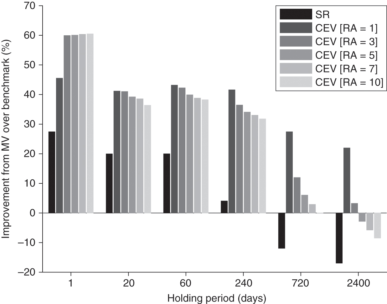
Finally, we illustrate the magnitude of the improvement in Figure 3. Here, we contrast these CEV improvements with the SR improvements in Table 1. The CEV improvement is larger across holding periods than the SR improvement: it is in the 30–60% range for up to one-year (240-day) holding periods, compared with the SR improvement of only about 5–25%. Finally, the improvement holds across risk-aversion assumptions. This lens is also more robust from an MPPM perspective and captures an important penalty for fat tails that the SR metric misses.
6 Conclusion
At the heart of so-called MV strategies lies a well-established and tantalizingly robust feature of financial markets: risk, as measured by volatility, is a time-variant feature of the return distribution, and unlike the expected return, a meaningful share of its time variation is forecastable by a surprisingly simple extrapolation of recently experienced volatility. Since the trade-off between risk and return is arguably the most fundamental concept of investment science, it is no surprise that MV has emerged as an investment framework. This framework capitalizes on risk forecastability by adjusting risk exposures inversely with predicted volatility in order to stabilize or manage the portfolio-level risk across time.
Our paper fills a gap in the literature by establishing stylized facts for historical MV performance by emphasizing the role of time. We use a very long-term series of US market returns, which enables us to probe for robustness along the dimension of historical periods, and we explicitly condition our results on holding periods. Our main conclusion is that MV strategies should be thought of in terms of their ability to mitigate tail risk first, rather than predominantly in terms of their potential for enhancements to risk-adjusted returns. For investor–practitioners who need to calibrate their own expectations toward MV, this distinction is critical. We establish the following stylized facts.
- (1)
When considering returns or SRs, MV enhances outcomes over the buy-and-hold benchmark, on average, but with variation in the sizing of the enhancements with holding period and across different starting historical periods.
- (2)
MV strategies remove fat tails (kurtosis) from the portfolio return as well as enhancing skewness. The return normalization feature of reducing kurtosis is inherently linked to the nature of the volatility stabilizing mechanism.
- (3)
When employing a utility framework to evaluate and compare MV strategies with the benchmark, the improvements in terms of the CEV are economically meaningful and show a larger relative improvement than those based on SRs. This evaluation framework also reflects the source of tangible value-add from MV strategies.
We encountered a number of areas that would benefit from additional research. Since MV strategies adjust equity market exposure in response to predicted volatility, they have an important connection to the literature on conditional equity market SRs. Much of this literature is dated earlier and focuses on business-cycle metrics for conditioning. Our sense is that more work can be done in terms of SRs conditional on predicted volatility, especially in terms of robustness to index and asset class, historical period, and holding period. Any robust conclusion on the pro- or countercyclicality of market SRs with respect to predicted volatility will naturally flow down to the merits of MV strategies that trade on those volatility predictions. Implementation considerations are a second area where much work is still left to be done. For investors who do measure performance against a buy-and-hold benchmark, MV can quickly introduce large amounts of tracking error to this benchmark, especially when using short-term forecasts that tend to work best for near-term volatility estimation. We believe that investment managers and applied researchers owe investors more thoughtful guidance on how to choose the “right-sized” exposure to MV strategies when a benchmark tracking error is being considered.
Declaration of interest
The authors report no conflicts of interest. The authors alone are responsible for the content and writing of the paper. This article is distributed under the terms of the Creative Commons Attribution 4.0 International License, https://creativecommons.org/licenses/by/4.0/.
Acknowledgements
T. Rowe Price has extensively researched MV for more than ten years and has implemented this investment approach for clients within internal and external strategies since December 2014. MV strategy solutions are proactively offered to suitable clients by qualified T. Rowe Price associates and are tailored by the multiasset investment team for client-specific objectives and constraints.
References
- Brandt, M. W., and Kang, Q. (2004). On the relationship between the conditional mean and volatility of stock returns: a latent VaR approach. Journal of Financial Economics 72, 217–257 (https://doi.org/10.1016/j.jfineco.2002.06.001).
- Clark, P. (1973). Subordinated stochastic process model with finite variance for speculative processes. Econometrica 41, 133–153 (https://doi.org/10.2307/1913889).
- Dopfel, F. E., and Ramkumar, S. R. (2013). Managed volatility strategies: applications to investment policy. Journal of Portfolio Management 30(1), 27–39 (https://doi.org/10.3905/jpm.2013.40.1.027).
- Dreyer, A. A., Harlow, R. L., Hubrich, S., and Page, S. (2016). Return of the quants: risk-based investing. CFA Institute Conference Proceedings Quarterly (Third Quarter), pp. 1–13 (https://doi.org/10.2469/cp.v33.n3.1).
- Ejara, D. D. (2016). Evaluating investments using higher moments. Modern Economy 7, 320–326 (https://doi.org/10.4236/me.2016.73035).
- Fleming, J., Kirby, C., and Ostdiek, B. (2001). The economic value of volatility timing. Journal of Finance LVI(1), 329–352 (https://doi.org/10.1111/0022-1082.00327).
- Fleming, J., Kirby, C., and Ostdiek, B. (2003). The economic value of volatility timing using “realized” volatility. Journal of Financial Economics 67(3), 473–509 (https://doi.org/10.1016/S0304-405X(02)00259-3).
- Goetzmann, W., Ingersoll, J., Spiegel, M., and Welch, I. (2007). Portfolio performance manipulation and manipulation-proof performance measures. Review of Financial Studies 20(5), 1503–1546 (https://doi.org/10.1093/rfs/hhm025).
- Hallerbach, W. G. (2012). A proof of the optimality of volatility weighting over time. The Journal of Investment Strategies 1(4), 87–99 (https://doi.org/10.21314/JOIS.2012.011).
- Hocquard, A., Ng, S., and Papageorgiu, N. (2013). A constant-volatility framework for managing tail risk. Journal of Portfolio Management 39(2), 28–40 (https://doi.org/10.3905/jpm.2013.39.2.028).
- Kinnel, R. (2015). Mind the gap 2015. Morningstar Manager Research, November 8.
- Kolanovic, M., and Wei, Z. (2013). Systematic strategies across asset classes: risk factor approach to investing and portfolio management. White Paper, JP Morgan.
- Lettau, M., and Ludvigson, S. (2010). Measuring and modeling variation in the risk–return tradeoff. In Handbook of Financial Econometrics, Ait-Sahalia, Y., and Hansen, L. P. (eds), pp. 617–690. Elsevier.
- Lundblad, C. (2007). The risk return tradeoff in the long run: 1863–2003. Journal of Financial Economics 85, 123–150 (https://doi.org/10.1016/j.jfineco.2006.06.003).
- Maillard, D. (2013). Manipulation-proof performance measure and the cost of tail risk. Working Paper, Social Science Research Network. URL: https://papers.ssrn.com/sol3/papers.cfm?abstract_id=2276050.
- Moreira, A., and Muir, T. (2016). How should investors respond to increases in volatility? Working Paper, AFA conference.
- Moreira, A., and Muir, T. (2017). Volatility managed portfolios. Journal of Finance 72(4), 1611–1644 (https://doi.org/10.1111/jofi.12513).
- Morningstar (2009). The Morningstar Rating methodology. Methodology Paper, June 30, Morningstar.
- Perchet, R., Leote de Cavalho, R., Heckel, T., and Moulin, P. (2014a). Inter-temporal risk parity: a constant volatility framework for equities and other asset classes. Working Paper, Social Science Research Network. URL: https://papers.ssrn.com/sol3/papers.cfm?abstract_id=2384583.
- Perchet, R., Leote de Cavalho, R., and Moulin, P. (2014b). Intertemporal risk parity: a constant volatility framework for factor investing. The Journal of Investment Strategies 4(1), 19–41 (https://doi.org/10.21314/JOIS.2015.036).
- Praetz, P. (1972). The distribution of share price changes. Journal of Business 45, 49–55 (https://doi.org/10.1086/295425).
- Press, S. J. (1967). A compound events model for security prices. Journal of Business 40, 317–335 (https://doi.org/10.1086/294980).
- Sun, H., Nelken, I., Han, G., and Guo, J. (2009). Error of VAR by overlapping intervals. Asia Risk, April, 50–55.
- Tang, Y., and Whitelaw, R. F. (2011). Time-varying Sharpe ratios and market timing. Quarterly Journal of Finance 1(3), 465–493 (https://doi.org/10.1142/S2010139211000122).
Only users who have a paid subscription or are part of a corporate subscription are able to print or copy content.
To access these options, along with all other subscription benefits, please contact info@risk.net or view our subscription options here: http://subscriptions.risk.net/subscribe
You are currently unable to print this content. Please contact info@risk.net to find out more.
You are currently unable to copy this content. Please contact info@risk.net to find out more.
Copyright Infopro Digital Limited. All rights reserved.
As outlined in our terms and conditions, https://www.infopro-digital.com/terms-and-conditions/subscriptions/ (point 2.4), printing is limited to a single copy.
If you would like to purchase additional rights please email info@risk.net
Copyright Infopro Digital Limited. All rights reserved.
You may share this content using our article tools. As outlined in our terms and conditions, https://www.infopro-digital.com/terms-and-conditions/subscriptions/ (clause 2.4), an Authorised User may only make one copy of the materials for their own personal use. You must also comply with the restrictions in clause 2.5.
If you would like to purchase additional rights please email info@risk.net